7 Week 7

Topic: Add Health data: variable creation and tabulation

This week’s lesson will provide more background on variable creation and tabulation of variables.

Download template.Rmd.txt as a template for this lesson. Save in in your working folder for the course, renamed to week_07.Rmd (with no .txt extension). Make any necessary changes to the YAML header.

Also make sure these packages are loaded:

pacman::p_load(
    tidyverse,
    magrittr,
    knitr,
    kableExtra,
    readstata13,
    haven,
    pdftools,
    curl,
    ggplot2,
    captioner
)

7.1 Creating value labels

“Labeled” data are important for documentation of data sets. The labels can apply to different objects, e.g., columns (as we saw in the column labels used to “decode” the data set in AHwave1_v1.dta, Section 1.6), or to individual values of variables, e.g., the attribute labels of the variable h1gi1m:

if (!exists("AHwave1_v1_haven")) {
    AHwave1_v1_haven <- haven::read_dta("http://staff.washington.edu/phurvitz/csde502_winter_2021/data/AHwave1_v1.dta")
}
attributes(AHwave1_v1_haven$h1gi1m)$labels %>%
    t() %>%
    t()

##               [,1]
## (1) January      1
## (2) February     2
## (3) March        3
## (4) April        4
## (5) May          5
## (6) June         6
## (7) July         7
## (8) August       8
## (9) September    9
## (10) October    10
## (11) November   11
## (12) December   12
## (96) Refused    96

Consider the difference between different file formats. Here we will save the data set, once as a CSV file and once an RDS file:

# temp dir
mytempdir <- tempdir()

write.csv(x = AHwave1_v1_haven, file = file.path(mytempdir, "AHwave1_v1_haven.csv"), row.names = FALSE)
saveRDS(object = AHwave1_v1_haven, file = file.path(mytempdir, "AHwave1_v1_haven.RDS"))

Then we will read them back in and investigate their structure. Here we are using a temporary folder, specified using the tmpdir() function. Each time an R session is started, a unique temporary folder is used. For the session used to create this document, the temporary dir is C:\59L.

First, read the CSV format:

AHwave1_v1_haven_csv <- read.csv(file = file.path(mytempdir, "AHwave1_v1_haven.csv"))

What kind of object is this?

is(AHwave1_v1_haven_csv)

## [1] "data.frame" "list"       "oldClass"   "vector"

It is a simple data frame. What attributes does this data set have? Here we list the attributes and enumerate the first 6 elements of each attribute:

AHwave1_v1_haven_csv %>%
    attributes() %>%
    map(~ head(.))

## $names
## [1] "aid"     "imonth"  "iday"    "iyear"   "bio_sex" "h1gi1m" 
## 
## $class
## [1] "data.frame"
## 
## $row.names
## [1] 1 2 3 4 5 6

There are three attributes, names, which are the individual column names; class, indicating this is a data frame, and row.names, in this case a serial number 1 .. n.

Do the columns have any attributes?

AHwave1_v1_haven_csv$h1gi1m %>%
    attributes()

## NULL

No, the columns have no attributes.

Now we will read in the RDS file:

AHwave1_v1_haven_rds <- readRDS(file = file.path(mytempdir, "AHwave1_v1_haven.RDS"))

What kind of object is this?

is(AHwave1_v1_haven_rds)

## [1] "tbl_df"     "tbl"        "data.frame" "list"       "oldClass"  
## [6] "vector"

It is a data frame–but an example of the tidyr subclass tibble; see the documentation.

What attributes does this data set have?

AHwave1_v1_haven_rds %>%
    attributes() %>%
    map(~ head(.))

## $class
## [1] "tbl_df"     "tbl"        "data.frame"
## 
## $row.names
## [1] 1 2 3 4 5 6
## 
## $label
## [1] "National Longitudinal Study of Adolescent to Adult Health (Add Health), 1994-200"
## 
## $names
## [1] "aid"     "imonth"  "iday"    "iyear"   "bio_sex" "h1gi1m"

The overall attributes are similar to the basic data frame, but there is an overall data set label, National Longitudinal Study of Adolescent to Adult Health (Add Health), 1994-200 (sic).

We can also look at the attributes of specific columns, here for h1gi1m:

AHwave1_v1_haven_rds$h1gi1m %>%
    attributes()

## $label
## [1] "S1Q1 BIRTH MONTH-W1"
## 
## $format.stata
## [1] "%13.0f"
## 
## $class
## [1] "haven_labelled" "vctrs_vctr"     "double"        
## 
## $labels
##   (1) January  (2) February     (3) March     (4) April       (5) May 
##             1             2             3             4             5 
##      (6) June      (7) July    (8) August (9) September  (10) October 
##             6             7             8             9            10 
## (11) November (12) December  (96) Refused 
##            11            12            96

Here we see that all of the original column attributes were preserved when the data set was saved in RDS format.

Importantly, saving a data set in CSV format loses any built-in metadata, whereas saving in RDS format maintains the built-in metadata. For other plain text formats, metadata will not be maintained; for other formats, it is worth determining whether such metadata are maintained. If metadata are not maintained in the file structure of the data set, it will be important to maintain the metadata in an external format (e.g., text, PDF). Note that the CSV format is the lingua franca of data transfer, and should be readable by any software, whereas the RDS format may not be readable by software other than R.

7.1.1 Creating factor variables

Factor variables are used in R to store categorical variables. These categorical variables can be nominal, in which each value is distinct and not ordered, such as race, classified as

White
Black/African American
American Indian
Asian/Pacific Islander
other

Factor variables can be ordered, where there is a difference in amount or intensity, such as self-reported health status:

Excellent
Very good
Good
Fair
Poor

Ordinal variables may or may not have equal intervals; for example, the “distance” between excellent and good health may not represent the same “distance” as the difference between good and fair health.

Structurally, factor variables are stored as integers that can be linked to text labels. Operationally, the use of factor variables is important in statistical modeling, so that the variables are handled correctly as being categorical.

Factor variables are created using the factor() or as_factor() functions. Here we will convert the self-reported general health variable (h1gh1) to a factor. First, let’s look at the variable:

AHwave1_v1_haven$h1gh1 %>%
    attributes()

## $label
## [1] "S3Q1 GENERAL HEALTH-W1"
## 
## $format.stata
## [1] "%14.0f"
## 
## $class
## [1] "haven_labelled" "vctrs_vctr"     "double"        
## 
## $labels
##  (1) Excellent  (2) Very good       (3) Good       (4) Fair       (5) Poor 
##              1              2              3              4              5 
##    (6) Refused (8) Don't know 
##              6              8

This shows that there are values 1 through 6 and 8, with coding indicated in the labels attribute. Using head() also reveals the structure of the variable, including the label for the variable itself as well as the coding of the variable values:

head(AHwave1_v1_haven$h1gh1)

## <labelled<double>[6]>: S3Q1 GENERAL HEALTH-W1
## [1] 3 4 4 4 3 3
## 
## Labels:
##  value          label
##      1  (1) Excellent
##      2  (2) Very good
##      3       (3) Good
##      4       (4) Fair
##      5       (5) Poor
##      6    (6) Refused
##      8 (8) Don't know

Here we convert the variable to a factor:

AHwave1_v1_haven$health <- factor(AHwave1_v1_haven$h1gh1)

What is the result? We can see from the first few values; head() presents the values as well as the levels.

# look at the first few values of the factor variable
head(AHwave1_v1_haven$health)

## [1] 3 4 4 4 3 3
## Levels: 1 2 3 4 5 6 8

Although the levels are in numerical order, there are no meaningful labels. We use the labels = argument to assign labels to each level. Simultaneously, because the factor is ordered in the same order as the alphanumeric ordering of the attributes, we can set the ordering based on those attributes. Finally, we reverse the order of the levels so that better health has a higher position in the order.

# extract the labels from the column attribute
health_levels <- AHwave1_v1_haven$h1gh1 %>%
    attributes() %>%
    extract2("labels") %>%
    names()

# create the factor variable and re-level it in reverse order
AHwave1_v1_haven$health <- factor(AHwave1_v1_haven$h1gh1,
    labels = health_levels,
    ordered = TRUE
) %>%
    fct_relevel(rev)

[Note that if the ordering is not alphanumeric, one should enter the list of values as ... labels = c("label1", "label2, ..., "labeln"), ordered = TRUE ... to enforce correct ordering.]

Let’s compare the two variables through simple tabulation. Here is the “raw” variable:

# "raw" variable
(tab_h1gh1 <- AHwave1_v1_haven %>%
    group_by(h1gh1) %>%
    summarise(n = n()))

## # A tibble: 7 x 2
##                h1gh1     n
##            <dbl+lbl> <int>
## 1 1 [(1) Excellent]   1847
## 2 2 [(2) Very good]   2608
## 3 3 [(3) Good]        1605
## 4 4 [(4) Fair]         408
## 5 5 [(5) Poor]          28
## 6 6 [(6) Refused]        3
## 7 8 [(8) Don't know]     5

The “raw” variable shows that it is a labeled, double precision variable (<dbl+lbl>).

Now the factor variable:

# factor variable
(tab_health <- AHwave1_v1_haven %>%
    group_by(health) %>%
    summarise(n = n()))

## # A tibble: 7 x 2
##   health             n
##   <ord>          <int>
## 1 (8) Don't know     5
## 2 (6) Refused        3
## 3 (5) Poor          28
## 4 (4) Fair         408
## 5 (3) Good        1605
## 6 (2) Very good   2608
## 7 (1) Excellent   1847

The counts are the same, but for the factor variable, the <ord> additionally indicates the ordering of health levels. Note that the order is different because (1) Excellent should have the highest numerical value–that is, in a statistical model, “Excellent” should have a greater value than “Poor.”

Bar plots also show the difference between the raw and factor variables. Figure 1 presents a bar plot from the raw variable.

ggplot(data = tab_h1gh1, aes(x = h1gh1, y = n)) +
    geom_bar(stat = "identity") +
    coord_flip()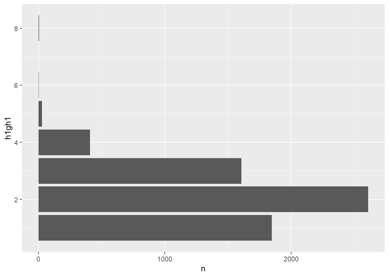

Figure 1: Bar plot from raw h1gh1 values

Because the numerical values have no special meaning, the bar plot uses its default method of displaying the axes. Figure 2 shows the bar plot created with the factor variable, with informative labels at the correct position on the axes.

ggplot(data = tab_health, mapping = aes(x = health, y = n)) +
    geom_bar(stat = "identity") +
    coord_flip()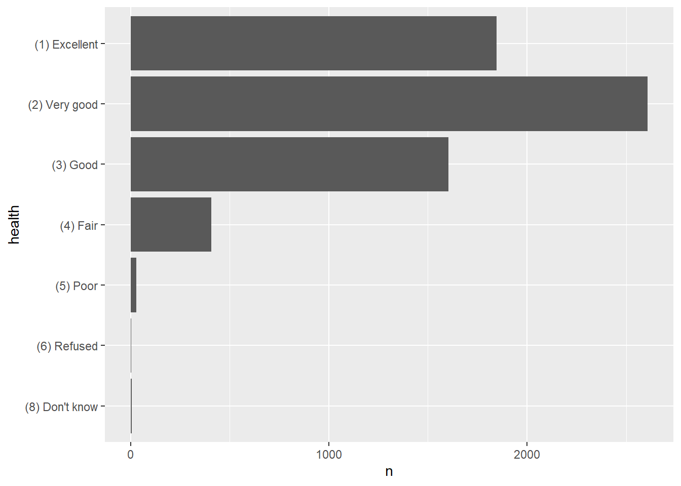

Figure 2: Bar plot from h1gh1 values as factors

One of the potential down sides to using factor variables is that using the text values requires additional code. For example, to select (filter()) a subset of records, there are two methods. The first method uses the label. In this case because the factor is ordered, it is possible to use an ordinal comparison. Any records with self-reported health less than or equal to “Very good” are selected. The tabulation shows that no “Excellent” records were selected.

# filter for Excellent or Very good
y <- AHwave1_v1_haven %>%
    filter(health <= "(2) Very good")

# tabulate
y %>%
    group_by(health) %>%
    summarise(n = n())

## # A tibble: 6 x 2
##   health             n
##   <ord>          <int>
## 1 (8) Don't know     5
## 2 (6) Refused        3
## 3 (5) Poor          28
## 4 (4) Fair         408
## 5 (3) Good        1605
## 6 (2) Very good   2608

The other method is to use as_numeric() to specify the underlying numerical values. In this case, because the value of 6 indicated Very good, we can filter for health %>% as.numeric() <= 6. However, it is critically important that the factor levels and values are known; in the original variable h1gh1, “Very good” had a value of 2, but in the re-ordered factor variable, “Very good” has a value of 6.

x <- AHwave1_v1_haven %>%
    filter(health %>% as.numeric() <= 6)

# tabulate
x %>%
    group_by(health) %>%
    summarise(n = n())

## # A tibble: 6 x 2
##   health             n
##   <ord>          <int>
## 1 (8) Don't know     5
## 2 (6) Refused        3
## 3 (5) Poor          28
## 4 (4) Fair         408
## 5 (3) Good        1605
## 6 (2) Very good   2608

Using unordered factor variables shows that more coding is generally involved in specifying values in filter() statements. For example, let’s create a factor variable for the interviewer’s observed single race variable:

# number of labels
nlabs <- length(unique(AHwave1_v1_haven$h1gi9))

# get the values, "as.numeric()"
obsrace_values <- AHwave1_v1_haven$h1gi9 %>%
    attributes() %>%
    extract2("labels") %>%
    as.numeric()

# get the labels, names()
obsrace_labels <- AHwave1_v1_haven$h1gi9 %>%
    attributes() %>%
    extract2("labels") %>%
    names()

# create the factor
AHwave1_v1_haven$obsrace <- factor(AHwave1_v1_haven$h1gi9,
    levels = obsrace_values,
    labels = obsrace_labels
)

Suppose we wanted to make a subset of only White and Black records, there are a few syntax methods:

Here, each value is explicitly named, using the | “or” operator

dat_wb1 <- AHwave1_v1_haven %>%
    filter(obsrace == "(1) White" |
        obsrace == "(2) Black/African American")

dat_wb1 %>%
    group_by(obsrace) %>%
    summarise(n = n())

## # A tibble: 2 x 2
##   obsrace                        n
##   <fct>                      <int>
## 1 (1) White                   4291
## 2 (2) Black/African American  1601

A different approach uses str_detect() with a regular expression to match any values of obsrace that contain the strings white or black in any upper/lower case combination.

dat_wb2 <- AHwave1_v1_haven %>%
    filter(str_detect(obsrace, regex("white|black", ignore_case = TRUE)))

dat_wb2 %>%
    group_by(obsrace) %>%
    summarise(n = n())

## # A tibble: 2 x 2
##   obsrace                        n
##   <fct>                      <int>
## 1 (1) White                   4291
## 2 (2) Black/African American  1601

Finally, if we know the numeric values representing the factors, we can use those directly, using requisite care in identifying the numeric values proxying for the factor levels:

dat_wb3 <- AHwave1_v1_haven %>%
    filter(obsrace %>% as.numeric() %in% c(1, 2))

dat_wb3 %>%
    group_by(obsrace) %>%
    summarise(n = n())

## # A tibble: 2 x 2
##   obsrace                        n
##   <fct>                      <int>
## 1 (1) White                   4291
## 2 (2) Black/African American  1601

The first method is the most verbose, requires the most code, and is probably the easiest to read. The other two methods may be easier to code (i.e., fewer keystrokes), but seem to be more difficult to read. There is often a trade-off between writing code that is quickly written and less easy to read versus code that is more methodically written but easier to read.

As above, care needs to be taken in saving the data set to a file. If the factor has text labels, those will be written as text by default to an output CSV file. When they are read back in, they will be treated as character values rather than ordered factors. For example, the health variable we created is an ordered factor:

str(AHwave1_v1_haven$health)

##  Ord.factor w/ 7 levels "(8) Don't know"<..: 5 4 4 4 5 5 4 7 6 6 ...

But when cycled through a write/read CSV cycle, the variable is not maintained as a factor.

write.csv(x = AHwave1_v1_haven, file = file.path(mytempdir, "foo.csv"), row.names = FALSE)

y <- read.csv(file.path(mytempdir, "foo.csv"))

str(y$health)

##  chr [1:6504] "(3) Good" "(4) Fair" "(4) Fair" "(4) Fair" "(3) Good" ...

Additional work would be needed to re-establish it as a factor. Fortunately, the alphanumeric sorting order of the character strings is also the logical order (i.e., (1) comes before (2) in alphanumeric order).

y$health <- factor(y$health,
    labels = y$health %>% unique() %>% sort(),
    ordered = TRUE
) %>% fct_rev()

head(y$health)

## [1] (3) Good (4) Fair (4) Fair (4) Fair (3) Good (3) Good
## 7 Levels: (8) Don't know < (6) Refused < (5) Poor < (4) Fair < ... < (1) Excellent

Without the numeric values preceding the text (e.g., (1), (2), …), the ordering would need to be explicitly set. For example, the vector in desired sorting order

"Excellent", "Very good", "Good", "Fair", "Poor", "Refused", "Don't know"

sorts as

"Excellent", "Very good", "Good", "Fair", "Poor", "Refused", "Don't know"

which is not the proper order of self-reported health.

To use our own specified labels, we need to include those in the desired order. Here we create a vector with specified labels in descending order matching the numeric values (i.e., 1 = “Excellent,” 2 = “Very good,” etc.), and then specify that vector in the labels argument:

health2labels <- c("Excellent", "Very good", "Good", "Fair", "Poor", "Refused", "Don't know")

y$health2 <- factor(y$h1gh1,
    labels = health2labels, 
    ordered = TRUE
) %>% fct_rev()

head(y$health2)

## [1] Good Fair Fair Fair Good Good
## 7 Levels: Don't know < Refused < Poor < Fair < Good < ... < Excellent

If you save the data set as RDS, the factor and other structures are maintained; here we see the factor levels are exactly as we set them earlier.

write_rds(x = AHwave1_v1_haven, file = file.path(mytempdir, "foo.Rds"))

z <- readRDS(file = file.path(mytempdir, "foo.Rds"))

head(z$health)

## [1] (3) Good (4) Fair (4) Fair (4) Fair (3) Good (3) Good
## 7 Levels: (8) Don't know < (6) Refused < (5) Poor < (4) Fair < ... < (1) Excellent

7.1.2 Creating attributes

In addition to creating factors, which can serve in some capacity as self-documenting (i.e., the value labels should be at least somewhat self-explanatory), we can create attributes as we have seen with the Stata .dta files.

Let’s start with the CSV file, which we know was stripped of its descriptive attributes:

y <- read.csv(file.path(mytempdir, "foo.csv"))

y %>%
    attributes() %>%
    map(~ head(.))

## $names
## [1] "aid"     "imonth"  "iday"    "iyear"   "bio_sex" "h1gi1m" 
## 
## $class
## [1] "data.frame"
## 
## $row.names
## [1] 1 2 3 4 5 6

First, an attribute of the data frame itself (the overall data frame label attribute):

attributes(y)$label <- "National Longitudinal Study of Adolescent to Adult Health (Add Health), 1994-2000 with some variable additions"

… which we can verify:

y %>%
    attributes() %>%
    extract("label")

## $label
## [1] "National Longitudinal Study of Adolescent to Adult Health (Add Health), 1994-2000 with some variable additions"

Next, attributes for the health and obsrace variables, documenting the variables and values. Here, for health we set this up as a factor using the sorted unique values of health from the CSV file. The factor is ordered and then reversed so that “Excellent” health has the highest value.

# label for health
attributes(y$health)$label <- "General health from public Add Health Wave 1 Section 3 question 1"

# labels for health
healthlevels <- unique(y$health) %>%
    sort()

# values for health
attributes(y$health)$levels <- healthlevels

# create the factor "health" with appropriate levels, order it and reverse the levels
#   so that Excellent is highest
y %<>% mutate(
    health =
        factor(health, levels = healthlevels, ordered = TRUE) %>%
            fct_rev()
)

We create the obsrace factor but because there is no inherent value hierarchy, we do not make this an ordered factor. We convert it to a factor for use in statistical models.

# label for obsrace
attributes(y$obsrace)$label <- "Interviewer observation of race from public Add Health Wave 1 Section 1 question 9"

# obsrace levels
obsracelevels <- unique(y$obsrace) %>%
    sort()

# values  for obsrace
attributes(y$obsrace)$levels <- obsracelevels

# create a factor
y %<>% mutate(
    obsrace = factor(obsrace, levels = obsracelevels)
)

Verify these were created:

y$health %>% attributes()

## $levels
## [1] "(8) Don't know" "(6) Refused"    "(5) Poor"       "(4) Fair"      
## [5] "(3) Good"       "(2) Very good"  "(1) Excellent" 
## 
## $class
## [1] "ordered" "factor"

head(y$health)

## [1] (3) Good (4) Fair (4) Fair (4) Fair (3) Good (3) Good
## 7 Levels: (8) Don't know < (6) Refused < (5) Poor < (4) Fair < ... < (1) Excellent

y$obsrace %>% attributes()

## $levels
## [1] "(1) White"                           "(2) Black/African American"         
## [3] "(3) American Indian/Native American" "(4) Asian/Pacific Islander"         
## [5] "(5) Other"                           "(6) Refused"                        
## [7] "(8) Don't know"                     
## 
## $class
## [1] "factor"

head(y$obsrace)

## [1] (2) Black/African American (2) Black/African American
## [3] (1) White                  (2) Black/African American
## [5] (2) Black/African American (2) Black/African American
## 7 Levels: (1) White ... (8) Don't know

The same caveats apply to saving the data frame to files, with respect to the various attributes and which attributes are saved and restored after a write/read cycle.

7.2 Tabulation

We have seen a few examples of tabulation in previous exercises (Sections 1.6.2.5, 2.2.4, 4.2.1.2.1). This section will give a more complete treatment using the Add Health data as an example.

7.2.1 Raw counts

The most basic tabulations simply give the count of observations in different strata. Those strata can be based on numeric ratio or interval data, using functions such as cut() or BAMMtools::getJenksBreaks(), nominal data (such as the Add Health interviewer’s observation of respondents’ single race), or ordinal data (such as the self-reported health status). We will use examples of each type of data.

First, this code will load the full Add Health data set, which includes additional variables not present in the data set we have used previously.

# download and unzip the larger data set
myUrl <- "http://staff.washington.edu/phurvitz/csde502_winter_2021/data/21600-0001-Data.dta.zip"

# zip file in $temp -- basename gets just the file name from the URL and not the URL path;
#   file.path stitches the tempdir() path to the file name
zipfile <- file.path(mytempdir, basename(myUrl))

# dta file in $temp
dtafile <- tools::file_path_sans_ext(zipfile)

# check if the dta file exists
if (!file.exists(dtafile)) {
    # if the dta file doesn't exist, check for the zip file
    # check if the zip file exists, download if necessary
    if (!file.exists(zipfile)) {
        curl::curl_download(url = myUrl, destfile = zipfile)
    }
    # unzip the downloaded zip file
    if (file.exists(zipfile)) {
        unzip(zipfile = zipfile, exdir = mytempdir)
    }
}

# if the data set has not been read, read it in
if (!exists("ahcomplete")) {
    ahcomplete <- haven::read_dta(dtafile)
}
# lowercase column names
colnames(ahcomplete) %<>% str_to_lower()

The metadata (variable names and labels) are presented in Table 1.

Table 1: Add Health large table variable names and labels

# create a data frame of the variable names and labels
ahcomplete_metadata <- bind_cols(
    varname = colnames(ahcomplete),
    varlabel = ahcomplete %>% map(~ attributes(.)$label) %>% unlist()
)

# print the table with DT::datatable for interactive display
DT::datatable(ahcomplete_metadata)

Let’s look at body mass index (BMI) data, which uses weight and height values. We find the variables representing weight and height from the metadata above. We need to determine if there are any invalid values:

attributes(ahcomplete$h1gh59a)$labels

##      (4) 4 feet      (5) 5 feet      (6) 6 feet    (96) Refused (98) Don't know 
##               4               5               6              96              98

attributes(ahcomplete$h1gh59b)$labels

##        (0) 0 inches          (1) 1 inch        (2) 2 inches        (3) 3 inches 
##                   0                   1                   2                   3 
##        (4) 4 inches        (5) 5 inches        (6) 6 inches        (7) 7 inches 
##                   4                   5                   6                   7 
##        (8) 8 inches        (9) 9 inches      (10) 10 inches      (11) 11 inches 
##                   8                   9                  10                  11 
##        (96) Refused     (98) Don't know (99) Not applicable 
##                  96                  98                  99

attributes(ahcomplete$h1gh60)$labels

##        (996) Refused     (998) Don't know (999) Not applicable 
##                  996                  998                  999

First, we need to select the variables representing feet and inches, then filter out invalid heights (> 90) and weights (> 900) identified above, and finally calculate height in m, weight in kg, and BMI (\(\frac{weight}{height^2}\)). For future use we will also select self-reported health and interviewer observed race as factors.

# make the data frame
htwt <- ahcomplete %>%
    # select columns
    select(
        feet = h1gh59a,
        inches = h1gh59b,
        weight_lb = h1gh60,
        health = h1gh1,
        obsrace = h1gi9
    ) %>%
    # filter for valid values
    filter(feet < 90 & inches < 90 & weight_lb < 900) %>%
    # calculate metric units and BMI
    mutate(
        height_m = (feet * 12 + inches) / 39.37008,
        weight_kg = weight_lb / 2.205,
        BMI = weight_kg / height_m^2
    )

# factor: get values and labels
healthvals <- htwt$health %>%
    attributes() %>%
    extract2("labels") %>%
    as.numeric()

healthlabs <- htwt$health %>%
    attributes() %>%
    extract2("labels") %>%
    names()

racevals <- htwt$obsrace %>%
    attributes() %>%
    extract2("labels") %>%
    as.numeric()

racelabs <- htwt$obsrace %>%
    attributes() %>%
    extract2("labels") %>%
    names()

# package the data frame up
htwt %<>%
    mutate(
        health = factor(health,
            levels = healthvals,
            labels = healthlabs
        ),
        obsrace = factor(obsrace,
            levels = racevals,
            labels = racelabs
        )
    )

A histogram (Figure 3 shows the distribution of BMI for the respondents with vertical lines at the 5th and 85th percentile. This range is generally considered “normal” or “healthy” according to the CDC, although for a sample with varying age, sex, height, and weight ranges, it is difficult to interpret. Nevertheless the cut points can serve the purpose of demonstration.

# get the 5th & 85th percentile
bmibreaks <- quantile(x = htwt$BMI, probs = c(0.05, 0.85))
ggplot(htwt, aes(x = BMI)) +
    geom_histogram(bins = 30) +
    geom_vline(xintercept = bmibreaks)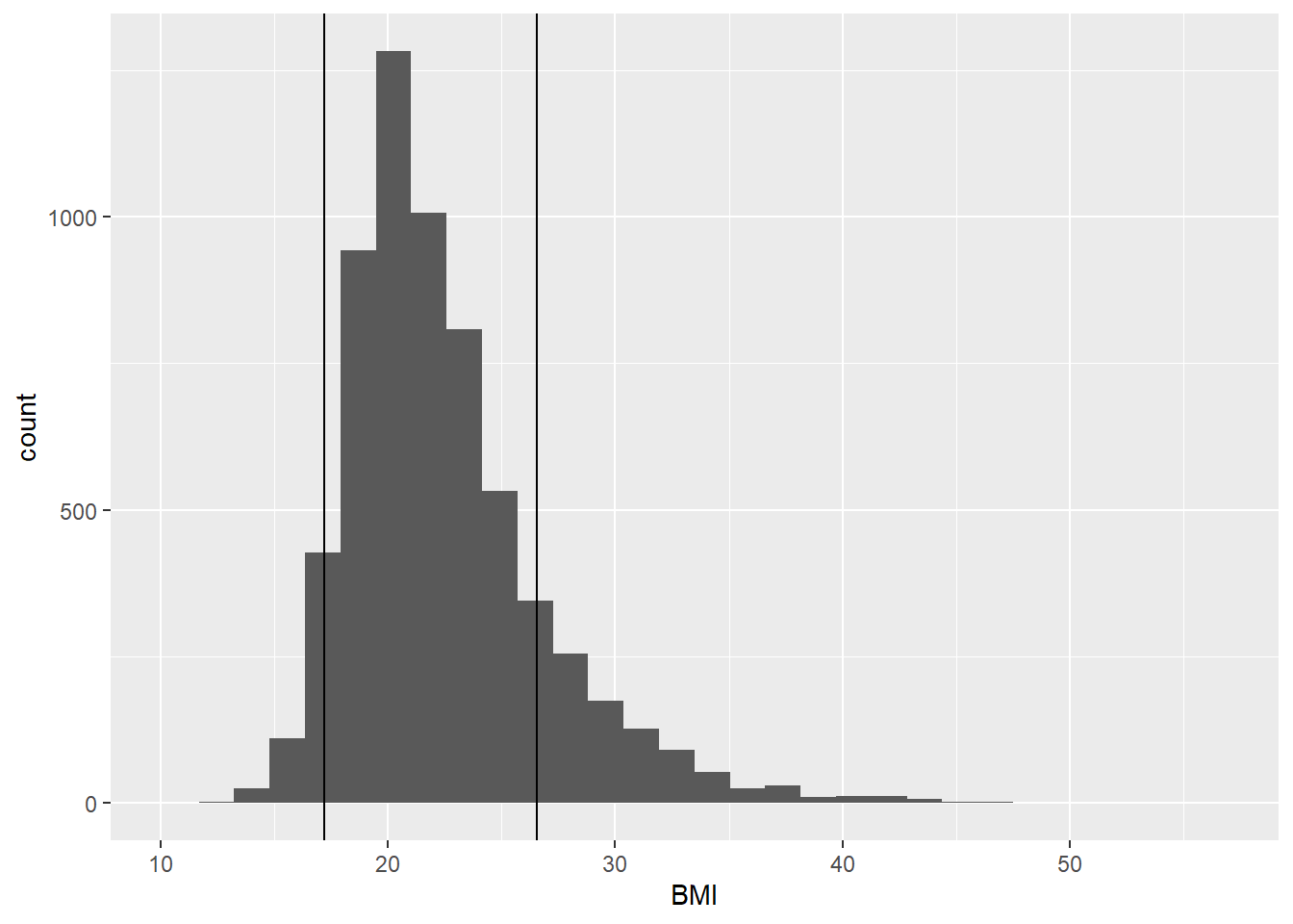

Figure 3: Histogram of BMI for Add Health cohort

We assign the BMI class using these cut points, with cut() breaks at the minimum, 5%, 85%, and maximum BMI, and also assign labels and set ordering:

htwt %<>%
    mutate(bmiclass = cut(
        x = BMI,
        breaks = c(min(BMI), bmibreaks, max(BMI)),
        labels = c("underweight", "normal", "overweight"),
        include.lowest = TRUE
    ) %>%
        factor(ordered = TRUE))

The tabulation of count of respondents by weight class can be generated with the base R function table() or dplyr functions group_by() and summarise() (Table 2.

# base R
table(htwt$bmiclass, useNA = "ifany")

## 
## underweight      normal  overweight 
##         324        5023         944

Table 2: Count by BMI class, Add Health cohort

# tidyR
htwt %>%
    group_by(bmiclass) %>%
    summarise(n = n()) %>%
    kable() %>%
    kable_styling(full_width = FALSE, position = "left", 
                  bootstrap_options = c("striped", "hover", "condensed", "responsive"))

bmiclass	n
underweight	324
normal	5023
overweight	944

For variables that are already nominal or ordinal factors, tabulations can be made directly. Because these were converted to factors, the correct labels will show, rather than simple numeric values. The tabulations will also be presented in descending order by label or level. Tabulation of self-reported health is in Table 3 and by race observed by interviewer in Table 4.

Table 3: Count by self-reported health class, Add Health cohort

htwt %>%
    group_by(health) %>%
    summarise(n = n()) %>%
    kable() %>%
    kable_styling(
        full_width = FALSE,
        position = "left",
        bootstrap_options = c("striped", "hover", "condensed", "responsive")
    )

health	n
Excellent	1803
Very good	2541
Good	1531
Fair	389
Poor	26
Don’t know	1

Table 4: Count by interviewer-observed race, Add Health cohort

htwt %>%
    group_by(obsrace) %>%
    summarise(n = n()) %>%
    kable() %>%
    kable_styling(
        full_width = FALSE, position = "left",
        bootstrap_options = c("striped", "hover", "condensed", "responsive")
    )

obsrace	n
White	4184
Black/African American	1525
American Indian/Native American	68
Asian/Pacific Islander	230
Other	280
Refused	1
Don’t know	3

7.2.2 Proportions/percentages

Proportions and percentages can be added to tabulations for greater interpretability. Using base R, the prop_table() function can be used as a wrapper around table() to generate proportions, optionally multiplying by 100 to generate a percentage. Remember to round as needed. For example:

round(prop.table(table(htwt$bmiclass)), 2)

## 
## underweight      normal  overweight 
##        0.05        0.80        0.15

round(prop.table(table(htwt$bmiclass)) * 100, 0)

## 
## underweight      normal  overweight 
##           5          80          15

Not surprisingly, the BMI classes show 5% underweight and 15% overweight, because that is how the stratification was defined.

The tidyR version requires a bit more coding but provides a more readable output. Because the percent sign is a special character, we enclose it in back ticks, %. Here we generate a tabulation of observed race (Table 4).

Table 5: Count by interviewer-observed race, Add Health cohort

htwt %>%
    group_by(obsrace) %>%
    summarise(n = n()) %>%
    mutate(`%` = n / sum(n) * 100) %>%
    mutate(`%` = `%` %>% round(1)) %>%
    kable() %>%
    kable_styling(
        full_width = FALSE, position = "left",
        bootstrap_options = c("striped", "hover", "condensed", "responsive")
    )

obsrace	n	%
White	4184	66.5
Black/African American	1525	24.2
American Indian/Native American	68	1.1
Asian/Pacific Islander	230	3.7
Other	280	4.5
Refused	1	0.0
Don’t know	3	0.0

7.2.3 Stratified tabulation

Tabulations can be generated using multiple variables. Here we will examine BMI and race as well as BMI and health. The percentages sum to 100 based on the order of the grouping.

Here, we see the relative percent of underweight, normal, and overweight within each race class (Table 6).

Table 6: Count by interviewer-observed race and BMI class, Add Health cohort

htwt %>%
    group_by(
        obsrace,
        bmiclass
    ) %>%
    summarise(n = n(), .groups = "drop_last") %>%
    mutate(`%` = n / sum(n) * 100) %>%
    mutate(`%` = `%` %>% round(1)) %>%
    kable() %>%
    kable_styling(
        full_width = FALSE, position = "left",
        bootstrap_options = c("striped", "hover", "condensed", "responsive")
    )

obsrace	bmiclass	n	%
White	underweight	234	5.6
White	normal	3389	81.0
White	overweight	561	13.4
Black/African American	underweight	52	3.4
Black/African American	normal	1188	77.9
Black/African American	overweight	285	18.7
American Indian/Native American	underweight	2	2.9
American Indian/Native American	normal	39	57.4
American Indian/Native American	overweight	27	39.7
Asian/Pacific Islander	underweight	20	8.7
Asian/Pacific Islander	normal	187	81.3
Asian/Pacific Islander	overweight	23	10.0
Other	underweight	16	5.7
Other	normal	216	77.1
Other	overweight	48	17.1
Refused	normal	1	100.0
Don’t know	normal	3	100.0

The table can also be presented with grouped rows. This code generates a named vector of the count of observed race by BMI class

# create the row groupings
(obsrace <- htwt %>%
    group_by(
        obsrace,
        bmiclass
    ) %>%
    summarise(n = n(), .groups = "drop_last") %>% 
    group_by(obsrace) %>% 
    summarise(n = n()) %>% 
    deframe())

##                           (1) White          (2) Black/African American 
##                                   3                                   3 
## (3) American Indian/Native American          (4) Asian/Pacific Islander 
##                                   3                                   3 
##                           (5) Other                         (6) Refused 
##                                   3                                   1 
##                      (8) Don't know 
##                                   1

The groups are then used in the pack_rows() function for grouped rows (Table 7).

Table 7: Count by interviewer-observed race and BMI class, Add Health cohort, percent by race

htwt %>%
    group_by(
        obsrace,
        bmiclass
    ) %>%
    summarise(n = n(), .groups = "drop_last") %>%
    mutate(`%` = n / sum(n) * 100) %>%
    mutate(`%` = `%` %>% round(1)) %>% 
    kable %>% 
    kable_styling(
        full_width = FALSE, position = "left",
        bootstrap_options = c("striped", "hover", "condensed", "responsive")
    ) %>% 
    pack_rows(index = obsrace)

obsrace	bmiclass	n	%
(1) White
White	underweight	234	5.6
White	normal	3389	81.0
White	overweight	561	13.4
(2) Black/African American
Black/African American	underweight	52	3.4
Black/African American	normal	1188	77.9
Black/African American	overweight	285	18.7
(3) American Indian/Native American
American Indian/Native American	underweight	2	2.9
American Indian/Native American	normal	39	57.4
American Indian/Native American	overweight	27	39.7
(4) Asian/Pacific Islander
Asian/Pacific Islander	underweight	20	8.7
Asian/Pacific Islander	normal	187	81.3
Asian/Pacific Islander	overweight	23	10.0
(5) Other
Other	underweight	16	5.7
Other	normal	216	77.1
Other	overweight	48	17.1
(6) Refused
Refused	normal	1	100.0
(8) Don’t know
Don’t know	normal	3	100.0

And here we see the relative percent of different race groups within each BMI class (Table 8.

Table 8: Count by interviewer-observed race and BMI class, Add Health cohort, percent by BMI class

htwt %>%
    group_by(
        bmiclass,
        obsrace
    ) %>%
    summarise(n = n(), .groups = "drop_last") %>%
    mutate(`%` = n / sum(n) * 100) %>%
    mutate(`%` = `%` %>% round(1)) %>%
    kable() %>%
    kable_styling(full_width = FALSE, position = "left",
                          bootstrap_options = c("striped", "hover", "condensed", "responsive")
)

bmiclass	obsrace	n	%
underweight	White	234	72.2
underweight	Black/African American	52	16.0
underweight	American Indian/Native American	2	0.6
underweight	Asian/Pacific Islander	20	6.2
underweight	Other	16	4.9
normal	White	3389	67.5
normal	Black/African American	1188	23.7
normal	American Indian/Native American	39	0.8
normal	Asian/Pacific Islander	187	3.7
normal	Other	216	4.3
normal	Refused	1	0.0
normal	Don’t know	3	0.1
overweight	White	561	59.4
overweight	Black/African American	285	30.2
overweight	American Indian/Native American	27	2.9
overweight	Asian/Pacific Islander	23	2.4
overweight	Other	48	5.1

Even though the n values are the same in the two tables (e.g., underweight \(\times\) White n = 234), the percentages are different due to grouping. That is, the percent of underweight persons among the White race stratum is different from the percent of White persons within the underweight stratum. Proper grouping is critical to answer specific questions about the data.

Another way to understand the data, preferred by some, would be to make a graph. For example, BMI by race as a facet grid bar graph (rfigure_nums(name = “bmibarfacet,” display = “cite”)`).

bmi_race <- htwt %>%
    group_by(
        obsrace,
        bmiclass
    ) %>%
    summarise(n = n(), .groups = "drop_last") %>%
    mutate(`%` = n / sum(n) * 100) %>%
    filter(!str_detect(obsrace, regex("refused|know", ignore_case = TRUE)))

ggplot(data = bmi_race, mapping = aes(x = bmiclass, y = `%`)) +
    geom_bar(stat = "identity") +
    theme(axis.text.x = element_text(angle = 90, vjust = 0.5, hjust = 1)) +
    facet_grid(~obsrace) +
    xlab("BMI class")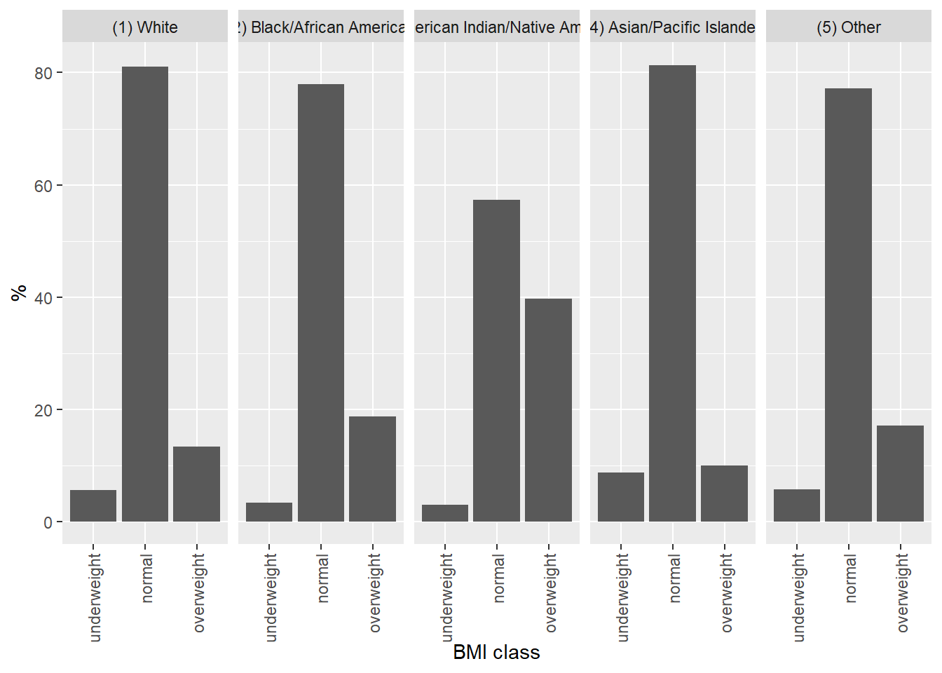

Figure 4: BMI class by race, Add Health cohort

Or as a stacked bar graph (Figure 5)

ggplot(data = bmi_race, mapping = aes(x = obsrace, y = `%`, fill = bmiclass)) +
    geom_bar(stat = "identity") +
    coord_flip() +
    scale_fill_discrete(name = "BMI class") +
    xlab("observed race")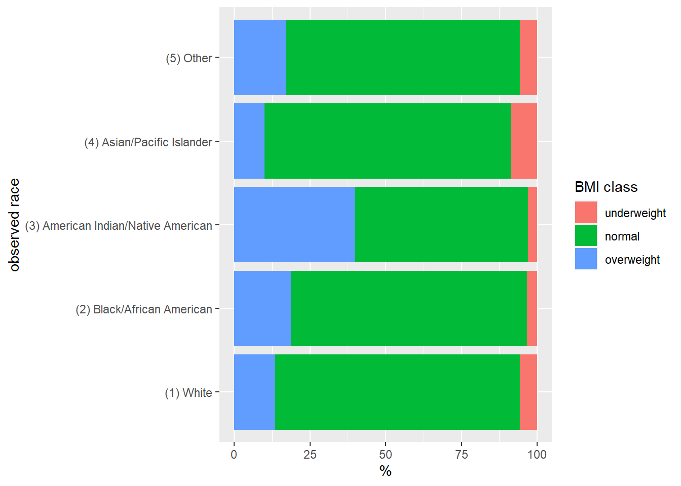

    #theme(axis.text.x = element_text(angle = 90, vjust = 0.5, hjust = 1))

Figure 5: BMI class by race, Add Health cohort

Rendered at 2022-03-12 10:47:23

7.3 Source code

File is at CSDE-TS1: R:/Project/CSDE502/2022/csde502-winter-2022-main/07-week07.Rmd.

7.3.1 R code used in this document

pacman::p_load(
    tidyverse,
    magrittr,
    knitr,
    kableExtra,
    readstata13,
    haven,
    pdftools,
    curl,
    ggplot2,
    captioner
)

table_nums <- captioner(prefix = "Table")
figure_nums <- captioner(prefix = "Figure")

# path to this file name
if (!interactive()) {
    fnamepath <- current_input(dir = TRUE)
    fnamestr <- paste0(Sys.getenv("COMPUTERNAME"), ": ", fnamepath)
} else {
    fnamepath <- ""
}
if (!exists("AHwave1_v1_haven")) {
    AHwave1_v1_haven <- haven::read_dta("http://staff.washington.edu/phurvitz/csde502_winter_2021/data/AHwave1_v1.dta")
}
attributes(AHwave1_v1_haven$h1gi1m)$labels %>%
    t() %>%
    t()
# temp dir
mytempdir <- tempdir()

write.csv(x = AHwave1_v1_haven, file = file.path(mytempdir, "AHwave1_v1_haven.csv"), row.names = FALSE)
saveRDS(object = AHwave1_v1_haven, file = file.path(mytempdir, "AHwave1_v1_haven.RDS"))
AHwave1_v1_haven_csv <- read.csv(file = file.path(mytempdir, "AHwave1_v1_haven.csv"))
is(AHwave1_v1_haven_csv)
AHwave1_v1_haven_csv %>%
    attributes() %>%
    map(~ head(.))
AHwave1_v1_haven_csv$h1gi1m %>%
    attributes()
AHwave1_v1_haven_rds <- readRDS(file = file.path(mytempdir, "AHwave1_v1_haven.RDS"))
is(AHwave1_v1_haven_rds)
AHwave1_v1_haven_rds %>%
    attributes() %>%
    map(~ head(.))
AHwave1_v1_haven_rds$h1gi1m %>%
    attributes()
AHwave1_v1_haven$h1gh1 %>%
    attributes()
head(AHwave1_v1_haven$h1gh1)
AHwave1_v1_haven$health <- factor(AHwave1_v1_haven$h1gh1)
# look at the first few values of the factor variable
head(AHwave1_v1_haven$health)
# extract the labels from the column attribute
health_levels <- AHwave1_v1_haven$h1gh1 %>%
    attributes() %>%
    extract2("labels") %>%
    names()

# create the factor variable and re-level it in reverse order
AHwave1_v1_haven$health <- factor(AHwave1_v1_haven$h1gh1,
    labels = health_levels,
    ordered = TRUE
) %>%
    fct_relevel(rev)
# "raw" variable
(tab_h1gh1 <- AHwave1_v1_haven %>%
    group_by(h1gh1) %>%
    summarise(n = n()))
# factor variable
(tab_health <- AHwave1_v1_haven %>%
    group_by(health) %>%
    summarise(n = n()))
ggplot(data = tab_h1gh1, aes(x = h1gh1, y = n)) +
    geom_bar(stat = "identity") +
    coord_flip()
ggplot(data = tab_health, mapping = aes(x = health, y = n)) +
    geom_bar(stat = "identity") +
    coord_flip()
# filter for Excellent or Very good
y <- AHwave1_v1_haven %>%
    filter(health <= "(2) Very good")

# tabulate
y %>%
    group_by(health) %>%
    summarise(n = n())
x <- AHwave1_v1_haven %>%
    filter(health %>% as.numeric() <= 6)

# tabulate
x %>%
    group_by(health) %>%
    summarise(n = n())
# number of labels
nlabs <- length(unique(AHwave1_v1_haven$h1gi9))

# get the values, "as.numeric()"
obsrace_values <- AHwave1_v1_haven$h1gi9 %>%
    attributes() %>%
    extract2("labels") %>%
    as.numeric()

# get the labels, names()
obsrace_labels <- AHwave1_v1_haven$h1gi9 %>%
    attributes() %>%
    extract2("labels") %>%
    names()

# create the factor
AHwave1_v1_haven$obsrace <- factor(AHwave1_v1_haven$h1gi9,
    levels = obsrace_values,
    labels = obsrace_labels
)
dat_wb1 <- AHwave1_v1_haven %>%
    filter(obsrace == "(1) White" |
        obsrace == "(2) Black/African American")

dat_wb1 %>%
    group_by(obsrace) %>%
    summarise(n = n())
dat_wb2 <- AHwave1_v1_haven %>%
    filter(str_detect(obsrace, regex("white|black", ignore_case = TRUE)))

dat_wb2 %>%
    group_by(obsrace) %>%
    summarise(n = n())
dat_wb3 <- AHwave1_v1_haven %>%
    filter(obsrace %>% as.numeric() %in% c(1, 2))

dat_wb3 %>%
    group_by(obsrace) %>%
    summarise(n = n())
str(AHwave1_v1_haven$health)
write.csv(x = AHwave1_v1_haven, file = file.path(mytempdir, "foo.csv"), row.names = FALSE)

y <- read.csv(file.path(mytempdir, "foo.csv"))

str(y$health)
y$health <- factor(y$health,
    labels = y$health %>% unique() %>% sort(),
    ordered = TRUE
) %>% fct_rev()

head(y$health)
health2labels <- c("Excellent", "Very good", "Good", "Fair", "Poor", "Refused", "Don't know")

y$health2 <- factor(y$h1gh1,
    labels = health2labels, 
    ordered = TRUE
) %>% fct_rev()

head(y$health2)
write_rds(x = AHwave1_v1_haven, file = file.path(mytempdir, "foo.Rds"))

z <- readRDS(file = file.path(mytempdir, "foo.Rds"))

head(z$health)
y <- read.csv(file.path(mytempdir, "foo.csv"))

y %>%
    attributes() %>%
    map(~ head(.))
attributes(y)$label <- "National Longitudinal Study of Adolescent to Adult Health (Add Health), 1994-2000 with some variable additions"
y %>%
    attributes() %>%
    extract("label")
# label for health
attributes(y$health)$label <- "General health from public Add Health Wave 1 Section 3 question 1"

# labels for health
healthlevels <- unique(y$health) %>%
    sort()

# values for health
attributes(y$health)$levels <- healthlevels

# create the factor "health" with appropriate levels, order it and reverse the levels
#   so that Excellent is highest
y %<>% mutate(
    health =
        factor(health, levels = healthlevels, ordered = TRUE) %>%
            fct_rev()
)
# label for obsrace
attributes(y$obsrace)$label <- "Interviewer observation of race from public Add Health Wave 1 Section 1 question 9"

# obsrace levels
obsracelevels <- unique(y$obsrace) %>%
    sort()

# values  for obsrace
attributes(y$obsrace)$levels <- obsracelevels

# create a factor
y %<>% mutate(
    obsrace = factor(obsrace, levels = obsracelevels)
)
y$health %>% attributes()
head(y$health)

y$obsrace %>% attributes()
head(y$obsrace)
# download and unzip the larger data set
myUrl <- "http://staff.washington.edu/phurvitz/csde502_winter_2021/data/21600-0001-Data.dta.zip"

# zip file in $temp -- basename gets just the file name from the URL and not the URL path;
#   file.path stitches the tempdir() path to the file name
zipfile <- file.path(mytempdir, basename(myUrl))

# dta file in $temp
dtafile <- tools::file_path_sans_ext(zipfile)

# check if the dta file exists
if (!file.exists(dtafile)) {
    # if the dta file doesn't exist, check for the zip file
    # check if the zip file exists, download if necessary
    if (!file.exists(zipfile)) {
        curl::curl_download(url = myUrl, destfile = zipfile)
    }
    # unzip the downloaded zip file
    if (file.exists(zipfile)) {
        unzip(zipfile = zipfile, exdir = mytempdir)
    }
}

# if the data set has not been read, read it in
if (!exists("ahcomplete")) {
    ahcomplete <- haven::read_dta(dtafile)
}
# lowercase column names
colnames(ahcomplete) %<>% str_to_lower()
# create a data frame of the variable names and labels
ahcomplete_metadata <- bind_cols(
    varname = colnames(ahcomplete),
    varlabel = ahcomplete %>% map(~ attributes(.)$label) %>% unlist()
)

# print the table with DT::datatable for interactive display
DT::datatable(ahcomplete_metadata)
attributes(ahcomplete$h1gh59a)$labels
attributes(ahcomplete$h1gh59b)$labels
attributes(ahcomplete$h1gh60)$labels
# make the data frame
htwt <- ahcomplete %>%
    # select columns
    select(
        feet = h1gh59a,
        inches = h1gh59b,
        weight_lb = h1gh60,
        health = h1gh1,
        obsrace = h1gi9
    ) %>%
    # filter for valid values
    filter(feet < 90 & inches < 90 & weight_lb < 900) %>%
    # calculate metric units and BMI
    mutate(
        height_m = (feet * 12 + inches) / 39.37008,
        weight_kg = weight_lb / 2.205,
        BMI = weight_kg / height_m^2
    )

# factor: get values and labels
healthvals <- htwt$health %>%
    attributes() %>%
    extract2("labels") %>%
    as.numeric()

healthlabs <- htwt$health %>%
    attributes() %>%
    extract2("labels") %>%
    names()

racevals <- htwt$obsrace %>%
    attributes() %>%
    extract2("labels") %>%
    as.numeric()

racelabs <- htwt$obsrace %>%
    attributes() %>%
    extract2("labels") %>%
    names()

# package the data frame up
htwt %<>%
    mutate(
        health = factor(health,
            levels = healthvals,
            labels = healthlabs
        ),
        obsrace = factor(obsrace,
            levels = racevals,
            labels = racelabs
        )
    )
# get the 5th & 85th percentile
bmibreaks <- quantile(x = htwt$BMI, probs = c(0.05, 0.85))
ggplot(htwt, aes(x = BMI)) +
    geom_histogram(bins = 30) +
    geom_vline(xintercept = bmibreaks)
htwt %<>%
    mutate(bmiclass = cut(
        x = BMI,
        breaks = c(min(BMI), bmibreaks, max(BMI)),
        labels = c("underweight", "normal", "overweight"),
        include.lowest = TRUE
    ) %>%
        factor(ordered = TRUE))
# base R
table(htwt$bmiclass, useNA = "ifany")
# tidyR
htwt %>%
    group_by(bmiclass) %>%
    summarise(n = n()) %>%
    kable() %>%
    kable_styling(full_width = FALSE, position = "left", 
                  bootstrap_options = c("striped", "hover", "condensed", "responsive"))
htwt %>%
    group_by(health) %>%
    summarise(n = n()) %>%
    kable() %>%
    kable_styling(
        full_width = FALSE,
        position = "left",
        bootstrap_options = c("striped", "hover", "condensed", "responsive")
    )
htwt %>%
    group_by(obsrace) %>%
    summarise(n = n()) %>%
    kable() %>%
    kable_styling(
        full_width = FALSE, position = "left",
        bootstrap_options = c("striped", "hover", "condensed", "responsive")
    )
round(prop.table(table(htwt$bmiclass)), 2)

round(prop.table(table(htwt$bmiclass)) * 100, 0)
htwt %>%
    group_by(obsrace) %>%
    summarise(n = n()) %>%
    mutate(`%` = n / sum(n) * 100) %>%
    mutate(`%` = `%` %>% round(1)) %>%
    kable() %>%
    kable_styling(
        full_width = FALSE, position = "left",
        bootstrap_options = c("striped", "hover", "condensed", "responsive")
    )
htwt %>%
    group_by(
        obsrace,
        bmiclass
    ) %>%
    summarise(n = n(), .groups = "drop_last") %>%
    mutate(`%` = n / sum(n) * 100) %>%
    mutate(`%` = `%` %>% round(1)) %>%
    kable() %>%
    kable_styling(
        full_width = FALSE, position = "left",
        bootstrap_options = c("striped", "hover", "condensed", "responsive")
    )
# create the row groupings
(obsrace <- htwt %>%
    group_by(
        obsrace,
        bmiclass
    ) %>%
    summarise(n = n(), .groups = "drop_last") %>% 
    group_by(obsrace) %>% 
    summarise(n = n()) %>% 
    deframe())
htwt %>%
    group_by(
        obsrace,
        bmiclass
    ) %>%
    summarise(n = n(), .groups = "drop_last") %>%
    mutate(`%` = n / sum(n) * 100) %>%
    mutate(`%` = `%` %>% round(1)) %>% 
    kable %>% 
    kable_styling(
        full_width = FALSE, position = "left",
        bootstrap_options = c("striped", "hover", "condensed", "responsive")
    ) %>% 
    pack_rows(index = obsrace)    
htwt %>%
    group_by(
        bmiclass,
        obsrace
    ) %>%
    summarise(n = n(), .groups = "drop_last") %>%
    mutate(`%` = n / sum(n) * 100) %>%
    mutate(`%` = `%` %>% round(1)) %>%
    kable() %>%
    kable_styling(full_width = FALSE, position = "left",
                          bootstrap_options = c("striped", "hover", "condensed", "responsive")
)
bmi_race <- htwt %>%
    group_by(
        obsrace,
        bmiclass
    ) %>%
    summarise(n = n(), .groups = "drop_last") %>%
    mutate(`%` = n / sum(n) * 100) %>%
    filter(!str_detect(obsrace, regex("refused|know", ignore_case = TRUE)))

ggplot(data = bmi_race, mapping = aes(x = bmiclass, y = `%`)) +
    geom_bar(stat = "identity") +
    theme(axis.text.x = element_text(angle = 90, vjust = 0.5, hjust = 1)) +
    facet_grid(~obsrace) +
    xlab("BMI class")
ggplot(data = bmi_race, mapping = aes(x = obsrace, y = `%`, fill = bmiclass)) +
    geom_bar(stat = "identity") +
    coord_flip() +
    scale_fill_discrete(name = "BMI class") +
    xlab("observed race")
    #theme(axis.text.x = element_text(angle = 90, vjust = 0.5, hjust = 1))
cat(readLines(fnamepath), sep = '\n')

7.3.2 Complete Rmd code

cat(readLines(fnamepath), sep = '\n')

# Week 7 {#week7}

```{r, echo=FALSE, warning=FALSE, message=FALSE}
pacman::p_load(
    tidyverse,
    magrittr,
    knitr,
    kableExtra,
    readstata13,
    haven,
    pdftools,
    curl,
    ggplot2,
    captioner
)

table_nums <- captioner(prefix = "Table")
figure_nums <- captioner(prefix = "Figure")

# path to this file name
if (!interactive()) {
    fnamepath <- current_input(dir = TRUE)
    fnamestr <- paste0(Sys.getenv("COMPUTERNAME"), ": ", fnamepath)
} else {
    fnamepath <- ""
}
```

<h2>Topic: Add Health data: variable creation and tabulation</h2>
This week's lesson will provide more background on variable creation and tabulation of variables.

Download [template.Rmd.txt](files/template.Rmd.txt) as a template for this lesson. Save in in your working folder for the course, renamed to `week_07.Rmd` (with no `.txt` extension). Make any necessary changes to the YAML header.

Also make sure these packages are loaded:

```
pacman::p_load(
    tidyverse,
    magrittr,
    knitr,
    kableExtra,
    readstata13,
    haven,
    pdftools,
    curl,
    ggplot2,
    captioner
)
```

## Creating value labels
"Labeled" data are important for documentation of data sets. The labels can apply to different objects, e.g., columns (as we saw in the column labels used to "decode" the data set in `AHwave1_v1.dta`, Section \@ref(tidyverse)), or to individual values of variables, e.g., the attribute `labels` of the variable `h1gi1m`:

```{r}
if (!exists("AHwave1_v1_haven")) {
    AHwave1_v1_haven <- haven::read_dta("http://staff.washington.edu/phurvitz/csde502_winter_2021/data/AHwave1_v1.dta")
}
attributes(AHwave1_v1_haven$h1gi1m)$labels %>%
    t() %>%
    t()
```

Consider the difference between different file formats. Here we will save the data set, once as a CSV file and once an RDS file:

```{r}
# temp dir
mytempdir <- tempdir()

write.csv(x = AHwave1_v1_haven, file = file.path(mytempdir, "AHwave1_v1_haven.csv"), row.names = FALSE)
saveRDS(object = AHwave1_v1_haven, file = file.path(mytempdir, "AHwave1_v1_haven.RDS"))
```

Then we will read them back in and investigate their structure. Here we are using a temporary folder, specified using the `tmpdir()` function. Each time an R session is started, a unique temporary folder is used. For the session used to create this document, the temporary dir is `r mytempdir`. 

First, read the CSV format:

```{r}
AHwave1_v1_haven_csv <- read.csv(file = file.path(mytempdir, "AHwave1_v1_haven.csv"))
```

What kind of object is this?

```{r}
is(AHwave1_v1_haven_csv)
```

It is a simple data frame. What attributes does this data set have? Here we list the attributes and enumerate the first 6 elements of each attribute:

```{r}
AHwave1_v1_haven_csv %>%
    attributes() %>%
    map(~ head(.))
```

There are three attributes, `names`, which are the individual column names; `class`, indicating this is a data frame, and `row.names`, in this case a serial number 1 .. n.

Do the columns have any attributes?

```{r}
AHwave1_v1_haven_csv$h1gi1m %>%
    attributes()
```

No, the columns have no attributes.

Now we will read in the RDS file:

```{r}
AHwave1_v1_haven_rds <- readRDS(file = file.path(mytempdir, "AHwave1_v1_haven.RDS"))
```

What kind of object is this?

```{r}
is(AHwave1_v1_haven_rds)
```

It is a data frame--but an example of the `tidyr` subclass `tibble`; see the [documentation](https://www.rdocumentation.org/packages/tibble).

What attributes does this data set have?

```{r}
AHwave1_v1_haven_rds %>%
    attributes() %>%
    map(~ head(.))
```

The overall attributes are similar to the basic data frame, but there is an overall data set label, ``r AHwave1_v1_haven_rds %>% attributes() %>% extract("label")`` (*sic*).

We can also look at the attributes of specific columns, here for `h1gi1m`:

```{r}
AHwave1_v1_haven_rds$h1gi1m %>%
    attributes()
```

Here we see that all of the original column attributes were preserved when the data set was saved in RDS format.

**Importantly**, saving a data set in CSV format loses any built-in metadata, whereas saving in RDS format maintains the built-in metadata. For other plain text formats, metadata will not be maintained; for other formats, it is worth determining whether such metadata are maintained. If metadata are not maintained in the file structure of the data set, it will be important to maintain the metadata in an external format (e.g., text, PDF). Note that the CSV format is the *lingua franca* of data transfer, and should be readable by any software, whereas the RDS format may not be readable by software other than R.

### Creating factor variables
Factor variables are used in R to store categorical variables. These categorical variables can be nominal, in which each value is distinct and *not* ordered, such as race, classified as 

* White
* Black/African American
* American Indian
* Asian/Pacific Islander
* other

Factor variables can be ordered, where there is a difference in amount or intensity, such as self-reported health status:

1. Excellent
1. Very good
1. Good
1. Fair
1. Poor

Ordinal variables may or may not have equal intervals; for example, the "distance" between excellent and good health may not represent the same "distance" as the difference between good and fair health.

Structurally, factor variables are stored as integers that can be linked to text labels. Operationally, __the use of factor variables is important in statistical modeling, so that the variables are handled correctly as being categorical__.

Factor variables are created using the `factor()` or `as_factor()` functions. Here we will convert the self-reported general health variable (`h1gh1`) to a factor. First, let's look at the variable:

```{r}
AHwave1_v1_haven$h1gh1 %>%
    attributes()
```

This shows that there are values 1 through 6 and 8, with coding indicated in the `labels` attribute. Using `head()` also reveals the structure of the variable, including the label for the variable itself as well as the coding of the variable values:

```{r}
head(AHwave1_v1_haven$h1gh1)
```


Here we convert the variable to a factor:

```{r}
AHwave1_v1_haven$health <- factor(AHwave1_v1_haven$h1gh1)
```

What is the result? We can see from the first few values; `head()` presents the values as well as the levels.

```{r}
# look at the first few values of the factor variable
head(AHwave1_v1_haven$health)
```

Although the levels are in numerical order, there are no meaningful labels. We use the `labels = ` argument to assign labels to each level. Simultaneously, because the factor is ordered in the same order as the alphanumeric ordering of the attributes, we can set the ordering based on those attributes. Finally, we reverse the order of the levels so that better health has a higher position in the order.

```{r}
# extract the labels from the column attribute
health_levels <- AHwave1_v1_haven$h1gh1 %>%
    attributes() %>%
    extract2("labels") %>%
    names()

# create the factor variable and re-level it in reverse order
AHwave1_v1_haven$health <- factor(AHwave1_v1_haven$h1gh1,
    labels = health_levels,
    ordered = TRUE
) %>%
    fct_relevel(rev)
```

_[Note that if the ordering is not alphanumeric, one should enter the list of values as `... labels = c("label1", "label2, ..., "labeln"), ordered = TRUE ...` to enforce correct ordering.]_

Let's compare the two variables through simple tabulation. Here is the "raw" variable:

```{r}
# "raw" variable
(tab_h1gh1 <- AHwave1_v1_haven %>%
    group_by(h1gh1) %>%
    summarise(n = n()))
```

The "raw" variable shows that it is a labeled, double precision variable (`<dbl+lbl>`). 

Now the factor variable:

```{r}
# factor variable
(tab_health <- AHwave1_v1_haven %>%
    group_by(health) %>%
    summarise(n = n()))
```

The counts are the same, but for the factor variable, the `<ord>` additionally indicates the ordering of health levels. Note that the order is different because `(1) Excellent` should have the highest numerical value--that is, in a statistical model, "Excellent" should have a greater value than "Poor".

Bar plots also show the difference between the raw and factor variables. `r figure_nums(name = "barplotraw", display = "cite")` presents a bar plot from the raw variable. 

```{r, warning=FALSE, message=FALSE}
ggplot(data = tab_h1gh1, aes(x = h1gh1, y = n)) +
    geom_bar(stat = "identity") +
    coord_flip()
```

*`r figure_nums(name = "barplotraw", caption = "Bar plot from raw h1gh1 values")`*

Because the numerical values have no special meaning, the bar plot uses its default method of displaying the axes. `r figure_nums(name = "barplotfac", display = "cite")` shows the bar plot created with the factor variable, with informative labels at the correct position on the axes.

```{r}
ggplot(data = tab_health, mapping = aes(x = health, y = n)) +
    geom_bar(stat = "identity") +
    coord_flip()
```

*`r figure_nums(name = "barplotfac", caption = "Bar plot from h1gh1 values as factors")`*


One of the potential down sides to using factor variables is that using the text values requires additional code. For example, to select (`filter()`) a subset of records, there are two methods. The first method uses the label. In this case because the factor is ordered, it is possible to use an ordinal comparison. Any records with self-reported health less than or equal to "Very good" are selected. The tabulation shows that no "Excellent" records were selected.

```{r}
# filter for Excellent or Very good
y <- AHwave1_v1_haven %>%
    filter(health <= "(2) Very good")

# tabulate
y %>%
    group_by(health) %>%
    summarise(n = n())
```

The other method is to use `as_numeric()` to specify the underlying numerical values. In this case, because the value of 6 indicated `Very good`, we can filter for `health %>% as.numeric() <= 6`.  However, it is critically important that the factor levels and values are known; in the original variable `h1gh1`, "Very good" had a value of 2, but in the re-ordered factor variable, "Very good" has a value of 6.

```{r}
x <- AHwave1_v1_haven %>%
    filter(health %>% as.numeric() <= 6)

# tabulate
x %>%
    group_by(health) %>%
    summarise(n = n())
```

Using unordered factor variables shows that more coding is generally involved in specifying values in `filter()` statements. For example, let's create a factor variable for the interviewer's observed single race variable:

```{r}
# number of labels
nlabs <- length(unique(AHwave1_v1_haven$h1gi9))

# get the values, "as.numeric()"
obsrace_values <- AHwave1_v1_haven$h1gi9 %>%
    attributes() %>%
    extract2("labels") %>%
    as.numeric()

# get the labels, names()
obsrace_labels <- AHwave1_v1_haven$h1gi9 %>%
    attributes() %>%
    extract2("labels") %>%
    names()

# create the factor
AHwave1_v1_haven$obsrace <- factor(AHwave1_v1_haven$h1gi9,
    levels = obsrace_values,
    labels = obsrace_labels
)
```

Suppose we wanted to make a subset of only White and Black records, there are a few syntax methods:

Here, each value is explicitly named, using the `|` "or" operator 

```{r}
dat_wb1 <- AHwave1_v1_haven %>%
    filter(obsrace == "(1) White" |
        obsrace == "(2) Black/African American")

dat_wb1 %>%
    group_by(obsrace) %>%
    summarise(n = n())
```

A different approach uses `str_detect()` with a regular expression to match any values of `obsrace` that contain the strings `white` or `black` in any upper/lower case combination.

```{r}
dat_wb2 <- AHwave1_v1_haven %>%
    filter(str_detect(obsrace, regex("white|black", ignore_case = TRUE)))

dat_wb2 %>%
    group_by(obsrace) %>%
    summarise(n = n())
```

Finally, if we know the numeric values representing the factors, we can use those directly, using requisite care in identifying the numeric values proxying for the factor levels:

```{r}
dat_wb3 <- AHwave1_v1_haven %>%
    filter(obsrace %>% as.numeric() %in% c(1, 2))

dat_wb3 %>%
    group_by(obsrace) %>%
    summarise(n = n())
```

The first method is the most verbose, requires the most code, and is probably the easiest to read. The other two methods may be easier to code (i.e., fewer keystrokes), but seem to be more difficult to read. There is often a trade-off between writing code that is quickly written and less easy to read versus code that is more methodically written but easier to read. 

As above, care needs to be taken in saving the data set to a file. If the factor has text labels, those will be written as text by default to an output CSV file. When they are read back in, they will be treated as character values rather than ordered factors. For example, the `health` variable we created is an ordered factor:

```{r}
str(AHwave1_v1_haven$health)
```

But when cycled through a write/read CSV cycle, the variable is not maintained as a factor.

```{r}
write.csv(x = AHwave1_v1_haven, file = file.path(mytempdir, "foo.csv"), row.names = FALSE)

y <- read.csv(file.path(mytempdir, "foo.csv"))

str(y$health)
```

Additional work would be needed to re-establish it as a factor. Fortunately, the alphanumeric sorting order of the character strings is also the logical order (i.e., `(1)` comes before `(2)` in alphanumeric order).

```{r}
y$health <- factor(y$health,
    labels = y$health %>% unique() %>% sort(),
    ordered = TRUE
) %>% fct_rev()

head(y$health)
```

Without the numeric values preceding the text (e.g., `(1)`, `(2)`, ...), the ordering would need to be explicitly set. For example, the vector in desired sorting order 

`"Excellent", "Very good", "Good", "Fair", "Poor", "Refused", "Don't know"` 

sorts as 

`"Excellent", "Very good", "Good", "Fair", "Poor", "Refused", "Don't know"`

which is not the proper order of self-reported health.

To use our own specified labels, we need to include those in the desired order. Here we create a vector with specified labels in descending order matching the numeric values (i.e., 1 = "Excellent", 2 = "Very good", etc.), and then specify that vector in the `labels` argument:

```{r}
health2labels <- c("Excellent", "Very good", "Good", "Fair", "Poor", "Refused", "Don't know")

y$health2 <- factor(y$h1gh1,
    labels = health2labels, 
    ordered = TRUE
) %>% fct_rev()

head(y$health2)
```

If you save the data set as RDS, the factor and other structures are maintained; here we see the factor levels are exactly as we set them earlier.

```{r}
write_rds(x = AHwave1_v1_haven, file = file.path(mytempdir, "foo.Rds"))

z <- readRDS(file = file.path(mytempdir, "foo.Rds"))

head(z$health)
```

### Creating attributes
In addition to creating factors, which can serve in some capacity as self-documenting (i.e., the value labels should be at least somewhat self-explanatory), we can create attributes as we have seen with the Stata `.dta` files.

Let's start with the CSV file, which we know was stripped of its descriptive attributes:

```{r}
y <- read.csv(file.path(mytempdir, "foo.csv"))

y %>%
    attributes() %>%
    map(~ head(.))
```

First, an attribute of the data frame itself (the overall data frame `label` attribute):

```{r}
attributes(y)$label <- "National Longitudinal Study of Adolescent to Adult Health (Add Health), 1994-2000 with some variable additions"
```

... which we can verify:

```{r}
y %>%
    attributes() %>%
    extract("label")
```

Next, attributes for the `health` and `obsrace` variables, documenting the variables and values. Here, for `health` we set this up as a factor using the sorted unique values of `health` from the CSV file. The factor is ordered and then reversed so that "Excellent" health has the highest value.

```{r}
# label for health
attributes(y$health)$label <- "General health from public Add Health Wave 1 Section 3 question 1"

# labels for health
healthlevels <- unique(y$health) %>%
    sort()

# values for health
attributes(y$health)$levels <- healthlevels

# create the factor "health" with appropriate levels, order it and reverse the levels
#   so that Excellent is highest
y %<>% mutate(
    health =
        factor(health, levels = healthlevels, ordered = TRUE) %>%
            fct_rev()
)
```

We create the `obsrace` factor but because there is no inherent value hierarchy, we do not make this an ordered factor. We convert it to a factor for use in statistical models.

```{r}
# label for obsrace
attributes(y$obsrace)$label <- "Interviewer observation of race from public Add Health Wave 1 Section 1 question 9"

# obsrace levels
obsracelevels <- unique(y$obsrace) %>%
    sort()

# values  for obsrace
attributes(y$obsrace)$levels <- obsracelevels

# create a factor
y %<>% mutate(
    obsrace = factor(obsrace, levels = obsracelevels)
)
```

Verify these were created:

```{r}
y$health %>% attributes()
head(y$health)

y$obsrace %>% attributes()
head(y$obsrace)
```

The same caveats apply to saving the data frame to files, with respect to the various attributes and which attributes are saved and restored after a write/read cycle.

## Tabulation
We have seen a few examples of tabulation in previous exercises (Sections \@ref(summarizingaggregating-data), \@ref(rmdtables), \@ref(default-values-for-arguments)). This section will give a more complete treatment using the Add Health data as an example.

### Raw counts
The most basic tabulations simply give the count of observations in different strata. Those strata can be based on numeric ratio or interval data, using functions such as `cut()` or `BAMMtools::getJenksBreaks()`, nominal data (such as the Add Health interviewer's observation of respondents' single race), or ordinal data (such as the self-reported health status). We will use examples of each type of data.

First, this code will load the full Add Health data set, which includes additional variables not present in the data set we have used previously.

```{r}
# download and unzip the larger data set
myUrl <- "http://staff.washington.edu/phurvitz/csde502_winter_2021/data/21600-0001-Data.dta.zip"

# zip file in $temp -- basename gets just the file name from the URL and not the URL path;
#   file.path stitches the tempdir() path to the file name
zipfile <- file.path(mytempdir, basename(myUrl))

# dta file in $temp
dtafile <- tools::file_path_sans_ext(zipfile)

# check if the dta file exists
if (!file.exists(dtafile)) {
    # if the dta file doesn't exist, check for the zip file
    # check if the zip file exists, download if necessary
    if (!file.exists(zipfile)) {
        curl::curl_download(url = myUrl, destfile = zipfile)
    }
    # unzip the downloaded zip file
    if (file.exists(zipfile)) {
        unzip(zipfile = zipfile, exdir = mytempdir)
    }
}

# if the data set has not been read, read it in
if (!exists("ahcomplete")) {
    ahcomplete <- haven::read_dta(dtafile)
}
# lowercase column names
colnames(ahcomplete) %<>% str_to_lower()
```

The metadata (variable names and labels) are presented in `r table_nums(name = "ahcompletemeta", display = "cite")`.

*`r table_nums(name = "ahcompletemeta", caption = "Add Health large table variable names and labels")`*

```{r}
# create a data frame of the variable names and labels
ahcomplete_metadata <- bind_cols(
    varname = colnames(ahcomplete),
    varlabel = ahcomplete %>% map(~ attributes(.)$label) %>% unlist()
)

# print the table with DT::datatable for interactive display
DT::datatable(ahcomplete_metadata)
```

\  

Let's look at body mass index (BMI) data, which uses weight and height values. We find the variables representing weight and height from the metadata above. We need to determine if there are any invalid values:

```{r}
attributes(ahcomplete$h1gh59a)$labels
attributes(ahcomplete$h1gh59b)$labels
attributes(ahcomplete$h1gh60)$labels
```

First, we need to select the variables representing feet and inches, then filter out invalid heights (> 90) and weights (> 900) identified above, and finally calculate height in m, weight in kg, and BMI ($\frac{weight}{height^2}$). For future use we will also select self-reported health and interviewer observed race as factors.

```{r}
# make the data frame
htwt <- ahcomplete %>%
    # select columns
    select(
        feet = h1gh59a,
        inches = h1gh59b,
        weight_lb = h1gh60,
        health = h1gh1,
        obsrace = h1gi9
    ) %>%
    # filter for valid values
    filter(feet < 90 & inches < 90 & weight_lb < 900) %>%
    # calculate metric units and BMI
    mutate(
        height_m = (feet * 12 + inches) / 39.37008,
        weight_kg = weight_lb / 2.205,
        BMI = weight_kg / height_m^2
    )

# factor: get values and labels
healthvals <- htwt$health %>%
    attributes() %>%
    extract2("labels") %>%
    as.numeric()

healthlabs <- htwt$health %>%
    attributes() %>%
    extract2("labels") %>%
    names()

racevals <- htwt$obsrace %>%
    attributes() %>%
    extract2("labels") %>%
    as.numeric()

racelabs <- htwt$obsrace %>%
    attributes() %>%
    extract2("labels") %>%
    names()

# package the data frame up
htwt %<>%
    mutate(
        health = factor(health,
            levels = healthvals,
            labels = healthlabs
        ),
        obsrace = factor(obsrace,
            levels = racevals,
            labels = racelabs
        )
    )
```

A histogram (`r figure_nums(name = "bmihist", display = "cite")` shows the distribution of BMI for the respondents with vertical lines at the 5th and 85th percentile. This range is generally considered "normal" or "healthy" according to the CDC, although for a sample with varying age, sex, height, and weight ranges, it is difficult to interpret. Nevertheless the cut points can serve the purpose of demonstration.

```{r}
# get the 5th & 85th percentile
bmibreaks <- quantile(x = htwt$BMI, probs = c(0.05, 0.85))
ggplot(htwt, aes(x = BMI)) +
    geom_histogram(bins = 30) +
    geom_vline(xintercept = bmibreaks)
```

\    
*`r figure_nums(name = "bmihist", caption = "Histogram of BMI for Add Health cohort")`*

We assign the BMI class using these cut points, with `cut()` breaks at the minimum, 5%, 85%, and maximum BMI, and also assign labels and set ordering:

```{r}
htwt %<>%
    mutate(bmiclass = cut(
        x = BMI,
        breaks = c(min(BMI), bmibreaks, max(BMI)),
        labels = c("underweight", "normal", "overweight"),
        include.lowest = TRUE
    ) %>%
        factor(ordered = TRUE))
```

The tabulation of count of respondents by weight class can be generated with the base R function `table()` or `dplyr` functions `group_by()` and `summarise()` (`r table_nums(name = "bmiclass", display = "cite")`.

```{r}
# base R
table(htwt$bmiclass, useNA = "ifany")
```

*`r table_nums(name = "bmiclass", caption = "Count by BMI class, Add Health cohort")`*

```{r}
# tidyR
htwt %>%
    group_by(bmiclass) %>%
    summarise(n = n()) %>%
    kable() %>%
    kable_styling(full_width = FALSE, position = "left", 
                  bootstrap_options = c("striped", "hover", "condensed", "responsive"))
```

For variables that are already nominal or ordinal factors, tabulations can be made directly. Because these were converted to factors, the correct labels will show, rather than simple numeric values. The tabulations will also be presented in descending order by label or level. Tabulation of self-reported health is in `r table_nums(name = "healthclass", display = "cite")` and by race observed by interviewer in `r table_nums(name = "obsraceclass", display = "cite")`.

*`r table_nums(name = "healthclass", caption = "Count by self-reported health class, Add Health cohort")`*

```{r}
htwt %>%
    group_by(health) %>%
    summarise(n = n()) %>%
    kable() %>%
    kable_styling(
        full_width = FALSE,
        position = "left",
        bootstrap_options = c("striped", "hover", "condensed", "responsive")
    )
```

*`r table_nums(name = "obsraceclass", caption = "Count by interviewer-observed race, Add Health cohort")`*

```{r}
htwt %>%
    group_by(obsrace) %>%
    summarise(n = n()) %>%
    kable() %>%
    kable_styling(
        full_width = FALSE, position = "left",
        bootstrap_options = c("striped", "hover", "condensed", "responsive")
    )
```

### Proportions/percentages
Proportions and percentages can be added to tabulations for greater interpretability. Using base R, the `prop_table()` function can be used as a wrapper around `table()` to generate proportions, optionally multiplying by 100 to generate a percentage. Remember to round as needed. For example:

```{r}
round(prop.table(table(htwt$bmiclass)), 2)

round(prop.table(table(htwt$bmiclass)) * 100, 0)
```

Not surprisingly, the BMI classes show 5% underweight and 15% overweight, because that is how the stratification was defined.

The `tidyR` version requires a bit more coding but provides a more readable output. Because the percent sign is a special character, we enclose it in back ticks, ``%``. Here we generate a tabulation of observed race (`r table_nums(name = "obsraceclass", display = "cite")`).

*`r table_nums(name = "obsraceclasspct", caption = "Count by interviewer-observed race, Add Health cohort")`*

```{r}
htwt %>%
    group_by(obsrace) %>%
    summarise(n = n()) %>%
    mutate(`%` = n / sum(n) * 100) %>%
    mutate(`%` = `%` %>% round(1)) %>%
    kable() %>%
    kable_styling(
        full_width = FALSE, position = "left",
        bootstrap_options = c("striped", "hover", "condensed", "responsive")
    )
```

### Stratified tabulation
Tabulations can be generated using multiple variables. Here we will examine BMI and race as well as BMI and health. The percentages sum to 100 based on the order of the grouping.

Here, we see the relative percent of underweight, normal, and overweight within each race class (`r table_nums(name = "obsracebmiclass", display = "cite")`).

*`r table_nums(name = "obsracebmiclass", caption = "Count by interviewer-observed race and BMI class, Add Health cohort")`*

```{r}
htwt %>%
    group_by(
        obsrace,
        bmiclass
    ) %>%
    summarise(n = n(), .groups = "drop_last") %>%
    mutate(`%` = n / sum(n) * 100) %>%
    mutate(`%` = `%` %>% round(1)) %>%
    kable() %>%
    kable_styling(
        full_width = FALSE, position = "left",
        bootstrap_options = c("striped", "hover", "condensed", "responsive")
    )
```

The table can also be presented with grouped rows. This code generates a named
vector of the count of observed race by BMI class

```{r}
# create the row groupings
(obsrace <- htwt %>%
    group_by(
        obsrace,
        bmiclass
    ) %>%
    summarise(n = n(), .groups = "drop_last") %>% 
    group_by(obsrace) %>% 
    summarise(n = n()) %>% 
    deframe())
```

The groups are then used in the `pack_rows()` function for grouped rows (`r table_nums(name = "obsracebmiclasspct", display = "cite")`).

*`r table_nums(name = "obsracebmiclasspct", caption = "Count by interviewer-observed race and BMI class, Add Health cohort, percent by race")`*

```{r}
htwt %>%
    group_by(
        obsrace,
        bmiclass
    ) %>%
    summarise(n = n(), .groups = "drop_last") %>%
    mutate(`%` = n / sum(n) * 100) %>%
    mutate(`%` = `%` %>% round(1)) %>% 
    kable %>% 
    kable_styling(
        full_width = FALSE, position = "left",
        bootstrap_options = c("striped", "hover", "condensed", "responsive")
    ) %>% 
    pack_rows(index = obsrace)    
```


And here we see the relative percent of different race groups within each BMI class (`r table_nums(name = "obsbmiraceclasspct", display = "cite")`. 

*`r table_nums(name = "obsbmiraceclasspct", caption = "Count by interviewer-observed race and BMI class, Add Health cohort, percent by BMI class")`*

```{r}
htwt %>%
    group_by(
        bmiclass,
        obsrace
    ) %>%
    summarise(n = n(), .groups = "drop_last") %>%
    mutate(`%` = n / sum(n) * 100) %>%
    mutate(`%` = `%` %>% round(1)) %>%
    kable() %>%
    kable_styling(full_width = FALSE, position = "left",
                          bootstrap_options = c("striped", "hover", "condensed", "responsive")
)
```

Even though the `n` values are the same in the two tables (e.g., underweight $\times$ White n = `r htwt %>% filter(str_detect(obsrace, "White") & str_detect(bmiclass, "under")) %>% nrow()`), the percentages are different due to grouping. That is, the percent of underweight persons among the White race stratum is different from the percent of White persons within the underweight stratum. Proper grouping is critical to answer specific questions about the data.

Another way to understand the data, preferred by some, would be to make a graph. For example, BMI by race as a facet grid bar graph (`r `figure_nums(name = "bmibarfacet", display = "cite")`).

```{r}
bmi_race <- htwt %>%
    group_by(
        obsrace,
        bmiclass
    ) %>%
    summarise(n = n(), .groups = "drop_last") %>%
    mutate(`%` = n / sum(n) * 100) %>%
    filter(!str_detect(obsrace, regex("refused|know", ignore_case = TRUE)))

ggplot(data = bmi_race, mapping = aes(x = bmiclass, y = `%`)) +
    geom_bar(stat = "identity") +
    theme(axis.text.x = element_text(angle = 90, vjust = 0.5, hjust = 1)) +
    facet_grid(~obsrace) +
    xlab("BMI class")
```

\    

*`r figure_nums(name = "bmibarfacet", caption = "BMI class by race, Add Health cohort")`*

Or as a stacked bar graph (`r figure_nums(name = "bmibarstack", display = "cite")`)

```{r}
ggplot(data = bmi_race, mapping = aes(x = obsrace, y = `%`, fill = bmiclass)) +
    geom_bar(stat = "identity") +
    coord_flip() +
    scale_fill_discrete(name = "BMI class") +
    xlab("observed race")
    #theme(axis.text.x = element_text(angle = 90, vjust = 0.5, hjust = 1))
```

\    
*`r figure_nums(name = "bmibarstack", caption = "BMI class by race, Add Health cohort")`*


<hr>
Rendered at <tt>`r Sys.time()`</tt>

## Source code
File is at `r fnamestr`.

### R code used in this document
```{r ref.label=knitr::all_labels(), echo=TRUE, eval=FALSE}
```

### Complete Rmd code
```{r comment=''}
cat(readLines(fnamepath), sep = '\n')
```

6 Week 6

8 Week 8