8 Week 8
Topic: Add Health data: variable creation and scale scoring
This week’s lesson will provide more background on variable creation and scale scoring. The scale scoring exercise will be used to create a single variable that represents how well respondents did overall on a subset of questions.
Download template.Rmd.txt as a template for this lesson. Save in in your working folder for the course, renamed to week_08.Rmd (with no .txt extension). Make any necessary changes to the YAML header.
Also load the following packages:
pacman::p_load(
    tidyverse,
    magrittr,
    knitr,
    kableExtra,
    haven,
    pdftools,
    curl,
    ggplot2,
    captioner
)
8.1 Scale scoring
We will be using data from the Knowledge Quiz. Download or open 21600-0001-Codebook_Questionnaire.pdf in a new window or tab and go to page 203, or search for the string Section 19: Knowledge Quiz.
We will be using the file AHwave1_v1.dta, which is downloaded and read in the following code chunk, along with presentation of the column names, labels, and values in Table 1.
Table 1: Metadata for AHwave1_v1.dta
dat <- haven::read_dta("http://staff.washington.edu/phurvitz/csde502_winter_2021/data/AHwave1_v1.dta")

metadata <- bind_cols(
    # variable name
    varname = colnames(dat),
    # label
    varlabel = lapply(dat, function(x) attributes(x)$label) %>%
        unlist(),
    # values
    varvalues = lapply(dat, function(x) attributes(x)$labels) %>%
        # names the variable label vector
        lapply(., function(x) names(x)) %>%
        # as character
        as.character() %>%
        # remove the c() construction
        str_remove_all("^c\\(|\\)$")
)

DT::datatable(metadata)
Questions H1KQ1A, H1KQ2A, …, H1KQ10A are factual questions about contraception that are administered to participants \(\ge\) age 15. We will be creating a single score that sums up all the correct answers across these questions for each participant \(\ge\) age 15. Because the set of questions is paired, with question “a” being the factual portion and “b” being the level of confidence, we want only those questions with column names ending with “a.”
8.1.1 Selecting specific columns
There are several ways of selecting the desired columns into a new data frame. There are two immediate objectives: filter for only those greater than 15 years of age, and select the desired columns.
The age cutoff can be seen in the value labels, which show that responses to H1KQ1a of value 7 represent those who are less than 15 years old.
attributes(dat$h1kq1a)$labels## (1) True (2) False <the correct answer>
## 1 2
## (6) Refused (7) Legitimate skip (less than 15)
## 6 7
## (8) Don't know (9) Not applicable
## 8 9Here is brute force approach to the filter and select:
# create a data frame of some columns and age >= 15
mydat_bruteforce <- dat %>%
    # drop those under 15 y
    filter(h1kq1a != 7) %>%
    # get answers
    select(
        aid, # subject ID
        h1kq1a,
        h1kq2a,
        h1kq3a,
        h1kq4a,
        h1kq5a,
        h1kq6a,
        h1kq7a,
        h1kq8a,
        h1kq9a,
        h1kq10a
    )
Although there were only 10 columns with this name pattern, what if there had been 30 or 50? You would not want to have to enter each column name separately. Not only would this be tedious, there would always be the possibility of making a keyboarding mistake.
Instead of the brute force approach, we can use the matches() function with a regular expression. The regular expression here is ^h1kq.*a$, which translates to “at the start of the string, match h1kq, then any number of any characters, then a followed by the end of the string.”
We check that both processes yielded the same result:
identical(mydat_bruteforce, mydat)## [1] TRUE8.1.2 Comparing participant answers to correct answers
Now that we have a data frame limited to the participants in the correct age range and only the questions we want, we need to set up tests for whether the questions were answered correctly or not. From the metadata we can see that for some questions, the correct answer was (1) true and for some, the correct answer was (2) false.
We need to look at questions in the metadata to create a vector of correct answers. For example, in the PDF see that the correct answer for H1KQ1A was (2) false.
# the correct answers from viewing the metadata
correct <- c(2, 1, 2, 2, 2, 2, 2, 1, 2, 2)
# make a named vector of the answers using the selected column names
names(correct) <- str_subset(string = names(mydat),
pattern = "h1kq.*a")
print(correct)## h1kq1a h1kq2a h1kq3a h1kq4a h1kq5a h1kq6a h1kq7a h1kq8a h1kq9a h1kq10a
## 2 1 2 2 2 2 2 1 2 2What we now need to do is compare this vector to a vector constructed of the answers in mydat. There are a few approaches that could be taken. A brute force approach could use a loop to iterate over each record in the answers, and for each record to iterate over each answer. This would need to iterate over nrow mydat rows and ncol(mydat) - 1 columns.
# time this
t0 <- Sys.time()
# make an output
ans_loop <- NULL
# iterate over rows
#testing:
#for(i in 1:3){
for(i in 1:nrow(mydat)){
# init a vector
Q <- NULL
# iterate over columns, ignoring the first "aid" column
for(j in 2:ncol(mydat)){
# get the value of the answer
ans_subj <- mydat[i, j]
# get the correct answer
ans_actual <- correct[j - 1]
# compare
cmp <- ans_actual == ans_subj
# append
Q <- c(Q, cmp)
}
# append
ans_loop <- rbind(ans_loop, Q)
}
# package it up nicely
ans_loop %<>% data.frame()
colnames(ans_loop) <- names(correct)
row.names(ans_loop) <- NULL
# timing
t1 <- Sys.time()
runtime_loop <- difftime(t1, t0, units = "secs") %>% as.numeric() %>% round(1)It took 20.3 s to run. This low performance is because the algorithm is visiting every cell and comparing one-by-on with a rotating value for the correct answer from the vector of correct answers. Each object is required to be handled separately in RAM as the process continues.
Another approach uses plyr::adply(), which runs a function over a set of rows. The plyr package contains a set of tools for splitting data, applying functions, and recombining.
# time this
t0 <- Sys.time()
ans_adply <- mydat %>%
select(-1) %>%
plyr::adply(.margins = 1,
function(x) x == correct)
# add the aid column
ans_adply <- data.frame(aid = mydat$aid, ans_adply)
t1 <- Sys.time()
runtime_adply <- difftime(t1, t0, units = "secs") %>% as.numeric() %>% round(1)The adply() version takes far less coding, but still took 19.9 s to run.
Yet another different approach compares the data frame of participant answers to the vector of correct answers. The correct answers vector will get recycled until all values have been processed. The problem with this method is that the comparison runs down columns rather than across rows.
The following hypothetical data set demonstrates the problem. Table 2 shows a pattern of “correct” values, and Table 3 shows a table of responses.
Table 2: A pattern of “correct” values
# make a pattern to match against
pat1 <- c(1, 2, 3, 4)
names(pat1) <- paste("question", 1:4, sep="_")
pat1 %>%
t() %>%
data.frame() %>%
kable(caption = 'A pattern of "correct" values') %>%
kable_styling(full_width = FALSE, position = "left")| question_1 | question_2 | question_3 | question_4 |
|---|---|---|---|
| 1 | 2 | 3 | 4 |
Table 3: A table of responses
# make a data frame to process
d1 <- cbind(rep(1, 3), rep(2, 3), rep(3,3), rep(4, 3)) %>%
data.frame()
names(d1) <- names(pat1)
d1 %>%
kable(caption = "A table of responses") %>%
kable_styling(full_width = FALSE, position = "left")| question_1 | question_2 | question_3 | question_4 |
|---|---|---|---|
| 1 | 2 | 3 | 4 |
| 1 | 2 | 3 | 4 |
| 1 | 2 | 3 | 4 |
We can test whether the pattern of correct answers (pat1) matches the first row of data (d1[1,]). The first row of data seems to match: Table 4.
Table 4: Matches for the first row
(pat1 == d1[1,]) %>%
kable(caption = "Matches for the first row") %>%
kable_styling(full_width = FALSE, position = "left") | question_1 | question_2 | question_3 | question_4 |
|---|---|---|---|
| TRUE | TRUE | TRUE | TRUE |
Next we test whether the pattern matches the entire table (d1 == pat1). The patterns do not match the overall table as might be expected (Table 5).
Table 5: Unexpected pattern matches
(d1 == pat1) %>%
kable(caption = "Unexpected pattern matches") %>%
kable_styling(full_width = FALSE, position = "left")| question_1 | question_2 | question_3 | question_4 |
|---|---|---|---|
| TRUE | FALSE | TRUE | FALSE |
| FALSE | FALSE | FALSE | FALSE |
| FALSE | TRUE | FALSE | TRUE |
In order to match the pattern to each row, a transpose is required. The following code performs the transpose, pattern match, and re-transpose, with results in Table 6.
Table 6: Expected pattern matches
# transpose, check for matching and transpose back
(d1 %>% t() == pat1) %>%
t() %>%
kable(caption = "Expected pattern matches") %>%
kable_styling(full_width = FALSE, position = "left") | question_1 | question_2 | question_3 | question_4 |
|---|---|---|---|
| TRUE | TRUE | TRUE | TRUE |
| TRUE | TRUE | TRUE | TRUE |
| TRUE | TRUE | TRUE | TRUE |
So the trick is to use a transpose (t()) to swap rows and columns. Then unlist() will enforce the correct ordering. After running the comparison, the data are transposed again to recreate the original structure.
# time this
t0 <- Sys.time()
# transpose and compare
ans_unlist <- mydat %>%
select(-1) %>%
t(.) %>%
unlist(.) == correct
# re-transpose and make a data frame
ans_unlist %<>%
t(.) %>%
data.frame()
# column names
colnames(ans_unlist) <- names(correct)
# aid
ans_unlist %<>%
mutate(aid = mydat$aid) %>%
select(aid, everything())
t1 <- Sys.time()
runtime_unlist <- difftime(t1, t0, units = "secs") %>% as.numeric() %>% round(2)This method took 0.02 s to complete.
Yet another method similarly uses the double transpose method.
# time this
t0 <- Sys.time()
# strip the ID column and transpose
z <- mydat %>%
select(-1) %>%
t()
# compare, transpose, and make a data frame
ans_tranpose <- (z == correct) %>%
t(.) %>%
data.frame() %>%
mutate(aid = mydat$aid) %>%
select(aid, everything())
t1 <- Sys.time()
runtime_transpose <- difftime(t1, t0, units = "secs") %>% as.numeric() %>% round(2)This method took 0.01 s to complete.
Finally, we will use a tidyverse approach, using pmap() from purrr. The commands will be shown as a series where each step is demonstrated separately. First we use pmap(~c(...)) which effectively creates a list where each element is a the vector of answers from a single row, i.e., each list element is the responses from a single participant. Here we drop the aid column because it is not present in the correct answers. Also a head() will run on only the first 6 rows.
## [[1]]
## <labelled<double>[10]>: S19Q1A SPERM DIES W/I 6 HOURS-W1
## h1kq1a h1kq2a h1kq3a h1kq4a h1kq5a h1kq6a h1kq7a h1kq8a h1kq9a h1kq10a
## 2 2 1 2 1 1 1 1 2 8
##
## Labels:
## value label
## 1 (1) True
## 2 (2) False <the correct answer>
## 6 (6) Refused
## 7 (7) Legitimate skip (less than 15)
## 8 (8) Don't know
## 9 (9) Not applicable
##
## [[2]]
## <labelled<double>[10]>: S19Q1A SPERM DIES W/I 6 HOURS-W1
## h1kq1a h1kq2a h1kq3a h1kq4a h1kq5a h1kq6a h1kq7a h1kq8a h1kq9a h1kq10a
## 2 2 1 1 2 2 2 1 2 2
##
## Labels:
## value label
## 1 (1) True
## 2 (2) False <the correct answer>
## 6 (6) Refused
## 7 (7) Legitimate skip (less than 15)
## 8 (8) Don't know
## 9 (9) Not applicable
##
## [[3]]
## <labelled<double>[10]>: S19Q1A SPERM DIES W/I 6 HOURS-W1
## h1kq1a h1kq2a h1kq3a h1kq4a h1kq5a h1kq6a h1kq7a h1kq8a h1kq9a h1kq10a
## 1 1 1 8 1 2 1 1 2 1
##
## Labels:
## value label
## 1 (1) True
## 2 (2) False <the correct answer>
## 6 (6) Refused
## 7 (7) Legitimate skip (less than 15)
## 8 (8) Don't know
## 9 (9) Not applicable
##
## [[4]]
## <labelled<double>[10]>: S19Q1A SPERM DIES W/I 6 HOURS-W1
## h1kq1a h1kq2a h1kq3a h1kq4a h1kq5a h1kq6a h1kq7a h1kq8a h1kq9a h1kq10a
## 2 2 2 2 2 1 1 1 2 1
##
## Labels:
## value label
## 1 (1) True
## 2 (2) False <the correct answer>
## 6 (6) Refused
## 7 (7) Legitimate skip (less than 15)
## 8 (8) Don't know
## 9 (9) Not applicable
##
## [[5]]
## <labelled<double>[10]>: S19Q1A SPERM DIES W/I 6 HOURS-W1
## h1kq1a h1kq2a h1kq3a h1kq4a h1kq5a h1kq6a h1kq7a h1kq8a h1kq9a h1kq10a
## 2 2 1 2 2 2 2 2 2 1
##
## Labels:
## value label
## 1 (1) True
## 2 (2) False <the correct answer>
## 6 (6) Refused
## 7 (7) Legitimate skip (less than 15)
## 8 (8) Don't know
## 9 (9) Not applicable
##
## [[6]]
## <labelled<double>[10]>: S19Q1A SPERM DIES W/I 6 HOURS-W1
## h1kq1a h1kq2a h1kq3a h1kq4a h1kq5a h1kq6a h1kq7a h1kq8a h1kq9a h1kq10a
## 2 1 1 2 2 2 2 1 2 1
##
## Labels:
## value label
## 1 (1) True
## 2 (2) False <the correct answer>
## 6 (6) Refused
## 7 (7) Legitimate skip (less than 15)
## 8 (8) Don't know
## 9 (9) Not applicableWe then use pmap(~c(...)==correct) to compare each participant’s answers against the correct answers, resulting in a list where each element is whether the participant’s answers were correct (also running on only the first 6 records).
## [[1]]
## [1] TRUE FALSE FALSE TRUE FALSE FALSE FALSE TRUE TRUE FALSE
##
## [[2]]
## [1] TRUE FALSE FALSE FALSE TRUE TRUE TRUE TRUE TRUE TRUE
##
## [[3]]
## [1] FALSE TRUE FALSE FALSE FALSE TRUE FALSE TRUE TRUE FALSE
##
## [[4]]
## [1] TRUE FALSE TRUE TRUE TRUE FALSE FALSE TRUE TRUE FALSE
##
## [[5]]
## [1] TRUE FALSE FALSE TRUE TRUE TRUE TRUE FALSE TRUE FALSE
##
## [[6]]
## [1] TRUE TRUE FALSE TRUE TRUE TRUE TRUE TRUE TRUE FALSETo wrap things up, we run on the entire data set, converting the output to a matrix.
t0 <- Sys.time()
ans_pmap <- mydat %>%
select(-aid) %>%
pmap(~c(...)==correct) %>%
do.call("rbind", .) %>%
data.frame()
# column names from mydat without the "aid" column
names(ans_pmap) <- names(mydat)[2:ncol(mydat)]
t1 <- Sys.time()
runtime_pmap <- difftime(t1, t0, units = "secs") %>% as.numeric() %>% round(3)The pmap() method took 13.005 seconds to run, not much better that the other methods.
Finally, we will use the base::sweep() method, which can be used to compare a vector against all rows or columns in a data frame. In order to use this function, the data frame needs to have the same number of rows (or columns) as the comparison vector. So any additional rows or columns need to be stripped. Because we may have additional columns (e.g., aid), those must be removed before running sweep(), then added back in again. Additionally, the result of sweep() is a matrix, so it needs to be converted to a data frame for greater functionality.
t0 <- Sys.time()
ans_sweep <- mydat %>%
# drop the aid column
select(-aid) %>%
# run the sweep
sweep(x = ., MARGIN = 2, STATS = correct, FUN = "==") %>%
# convert to data frame
data.frame()
t1 <- Sys.time()
runtime_sweep <- difftime(t1, t0, units = "secs") %>% as.numeric() %>% round(3)The sweep() method took 0.009 s.
We should check that the methods all gave identical answers. This compares ans_loop with each of the outputs of the other methods (Table 7). The exercise is intended to show that there are frequently many different ways to achieve the same end goal, and some methods are more efficient than others. One can always take a subset of data and test different methods for the fastest run times before running a time-consuming process on a complete data set.
Table 7: Run times of row-matching to correct answers
# make a data frame summarizing the results of each method
# methods
method <- c("loop", "adply", "transpose", "unlist", "pmap")
# run times
run_time <- c(runtime_loop, runtime_adply, runtime_transpose, runtime_unlist, runtime_pmap) %>% round(2)
# comparisons
match <- Vectorize(identical, 'x')(list(ans_loop, ans_adply, ans_tranpose, ans_unlist, ans_pmap), ans_loop)
# a single data frame
comparisons <- data.frame(method, run_time, match) %>%
arrange(run_time)
# print
comparisons %>%
kable() %>%
kable_styling(full_width = FALSE, position = "left") | method | run_time | match |
|---|---|---|
| transpose | 0.01 | FALSE |
| unlist | 0.02 | FALSE |
| pmap | 13.01 | TRUE |
| adply | 19.90 | FALSE |
| loop | 20.30 | TRUE |
8.1.3 Scoring across columns
Now that we have a data frame indicating for each participant whether they answered each question correctly, we can total the number of correct answers for each participant. The rowSums() function allows sums across rows. Because the logical values are automatically converted to numerical values (TRUE = 1; FALSE = 0), the sums provide the total number of correct answers per participant. Also because the data frame only consists of answers 1 .. 10, we can use an unqualified rowSums(), otherwise it would be necessary to specify which columns would be included by either position or column name.
We also bring the subject identifier (aid) back in and reorder the columns with select(). Note that after the specified aid and total h1kqNa_sum columns, we can use everything() to select the remainder of the columns.
ans_loop %<>%
# calculate the rowSums
mutate(h1kqNa_sum = rowSums(.)) %>%
# bring the ID back in
mutate(aid = mydat$aid) %>%
# reorder columns
select(aid, h1kqNa_sum, everything())To show differences in total score by sex, we can join the main data back using the aid identifier and create a simple graph. Figure 8.1 shows that more females than males had overall higher counts of correct scores on the Knowledge Quiz.
ans_loop %<>%
left_join(dat, by = "aid") %>%
mutate(
sex = case_when(
bio_sex == 1 ~ 'male',
bio_sex == 2 ~ 'female'
)
)
ggplot(data = ans_loop, mapping = aes(x = h1kqNa_sum))+
geom_bar() +
facet_grid(sex ~ .) +
xlab("correct answers on Knowledge Quiz") +
scale_x_continuous(breaks=0:10)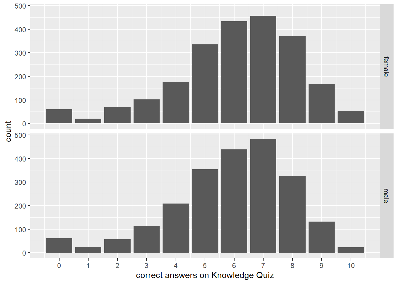
Figure 8.1: Histogram of count of correct answers on Knowledge Quiz stratified by sex of respondent
8.2 Reordering values
Sometimes variables are provided in the reverse order of what you might want. For example, the answers pertaining to confidence in the Knowledge Quiz are in this specific order:
attributes(dat$h1kq1b)$labels %>% t() %>% t() %>% data.frame()## .
## (1) Very 1
## (2) Moderately 2
## (3) Slightly 3
## (4) Not at all 4
## (6) Refused 6
## (7) Legitimate skip (less than 15) 7
## (8) Don't know 8
## (9) Not applicable 9To come up with a scale score for these, it would be better to have Very valued as a 4 and Not at all as a 1 so that row-wise sums would yield higher values for those who were more confident in many answers (ignoring answers that cannot be scaled, i.e., refused, skipped, don’t know, not applicable). One could use the existing values, but then the interpretation of an overall confidence score might be difficult, with the most confidence for the lowest overall score.
Changing these values is quite straightforward. The case_when() function can be used. case_when() uses the structure var == input_value ~ output_value, where var is the column name, input_value is the selected value, and output_value is the reassigned value. Any additional cases that were not addressed specifically can be handled with TRUE ~ output_value.
# for comparison, make a backup data frame
datbak <- dat2 <- dat
# reassign values
dat %<>%
mutate(h1kq1b =
case_when(
# main changes
h1kq1b == 4 ~ 1,
h1kq1b == 3 ~ 2,
h1kq1b == 2 ~ 3,
h1kq1b == 1 ~ 4,
# anything that is not in the above list gets its original value
TRUE ~ as.numeric(h1kq1b))
)Let’s see what these values look like now. The first records before reordering:
head(datbak$h1kq1b)## <labelled<double>[6]>: S19Q1B CONFIDENT 1A IS CORRECT-W1
## [1] 1 3 2 3 1 7
##
## Labels:
## value label
## 1 (1) Very
## 2 (2) Moderately
## 3 (3) Slightly
## 4 (4) Not at all
## 6 (6) Refused
## 7 (7) Legitimate skip (less than 15)
## 8 (8) Don't know
## 9 (9) Not applicable… and the first few records after reordering:
head(dat$h1kq1b)## [1] 4 2 3 2 4 7It is a bit more awkward to perform this kind of reordering operation on multiple columns. One might be tempted to use a brute force method by copy/paste/edit to have a large set of case_when() functions for each column, but this would be tedious and error-prone.
Using the mutate_at() function can help through the use of regular expression pattern matching for column names. The same function will be performed on multiple columns. Here we use a similar regular expression to find the columns representing confidence in answers to the Knowledge Quiz (h1kq.*b = “starts with h1kq, then has any numbner of characters, then has a b”) to perform the operation on any columns with names matching the regular expression pattern. The use of the dot (.) is shorthand for “the current object” which in this case is the specified column in a virtual loop over columns matching in name with the pattern.
dat2 %<>%
mutate_at(.vars = vars(matches("h1kq.*b")),
list(
~case_when(
. == 4 ~ 1,
. == 3 ~ 2,
. == 2 ~ 3,
. == 1 ~ 4,
TRUE ~ as.numeric(.)
)
)
)For the sake of comparison to show that the single bit of code acted on multiple columns. Two variables are shown in Table 8, with the frequencies of the original confidence values (orig) and the reordered confidence values (modified).
orig1 <- table(datbak$h1kq1b) %>% data.frame()
mod1 <- table(dat$h1kq1b) %>% data.frame()
orig2 <- table(datbak$h1kq2b) %>% data.frame()
mod2 <- table(dat$h1kq2b) %>% data.frame()Table 8: Confidence in correctness of answer
reordered <- cbind(orig1, mod1, orig2, mod2)
reordered %>%
kable() %>%
kable_styling(full_width = FALSE, position = "left") %>%
add_header_above(rep(c("original" = 2, "modified" = 2), 2)) %>%
add_header_above(c("h1kq1b" = 4, "h1kq2b" = 4))| Var1 | Freq | Var1 | Freq | Var1 | Freq | Var1 | Freq |
|---|---|---|---|---|---|---|---|
| 1 | 1070 | 1 | 373 | 1 | 1658 | 1 | 1658 |
| 2 | 1723 | 2 | 1109 | 2 | 1542 | 2 | 1542 |
| 3 | 1109 | 3 | 1723 | 3 | 800 | 3 | 800 |
| 4 | 373 | 4 | 1070 | 4 | 289 | 4 | 289 |
| 6 | 27 | 6 | 27 | 6 | 32 | 6 | 32 |
| 7 | 2039 | 7 | 2039 | 7 | 2039 | 7 | 2039 |
| 8 | 162 | 8 | 162 | 8 | 143 | 8 | 143 |
| 9 | 1 | 9 | 1 | 9 | 1 | 9 | 1 |
For example, the original value of 1 had a count of 1070 but the transformed value is 4 with the same count. Now that the values are reordered, they can be used in multiple-column scale scoring as demonstrated above.
Rendered at 2022-03-12 10:48:21
8.3 Source code
File is at CSDE-TS1: R:/Project/CSDE502/2022/csde502-winter-2022-main/08-week08.Rmd.
8.3.1 R code used in this document
pacman::p_load(
tidyverse,
magrittr,
knitr,
kableExtra,
haven,
pdftools,
curl,
ggplot2,
captioner
)
table_nums <- captioner(prefix = "Table")
figure_nums <- captioner(prefix = "Figure")
# path to this file name
if (!interactive()) {
fnamepath <- current_input(dir = TRUE)
fnamestr <- paste0(Sys.getenv("COMPUTERNAME"), ": ", fnamepath)
} else {
fnamepath <- ""
}
dat <- haven::read_dta("http://staff.washington.edu/phurvitz/csde502_winter_2021/data/AHwave1_v1.dta")
metadata <- bind_cols(
# variable name
varname = colnames(dat),
# label
varlabel = lapply(dat, function(x) attributes(x)$label) %>%
unlist(),
# values
varvalues = lapply(dat, function(x) attributes(x)$labels) %>%
# names the variable label vector
lapply(., function(x) names(x)) %>%
# as character
as.character() %>%
# remove the c() construction
str_remove_all("^c\\(|\\)$")
)
DT::datatable(metadata)
attributes(dat$h1kq1a)$labels
# create a data frame of some columns and age >= 15
mydat_bruteforce <- dat %>%
# drop those under 15 y
filter(h1kq1a != 7) %>%
# get answers
select(
aid, # subject ID
h1kq1a,
h1kq2a,
h1kq3a,
h1kq4a,
h1kq5a,
h1kq6a,
h1kq7a,
h1kq8a,
h1kq9a,
h1kq10a
)
mydat <- dat %>%
    filter(h1kq1a != 7) %>%
    select(
        aid,
        matches("h1kq.*a")
    )
identical(mydat_bruteforce, mydat)
# the correct answers from viewing the metadata
correct <- c(2, 1, 2, 2, 2, 2, 2, 1, 2, 2)

# make a named vector of the answers using the selected column names
names(correct) <- str_subset(string = names(mydat),
                             pattern = "h1kq.*a")

print(correct)
# time this
t0 <- Sys.time()

# make an output
ans_loop <- NULL

# iterate over rows
#testing:
#for(i in 1:3){
for(i in 1:nrow(mydat)){
    # init a vector
    Q <- NULL
    # iterate over columns, ignoring the first "aid" column
    for(j in 2:ncol(mydat)){
        # get the value of the answer
        ans_subj <- mydat[i, j]
        # get the correct answer
        ans_actual <- correct[j - 1]
        # compare
        cmp <- ans_actual == ans_subj
        # append
        Q <- c(Q, cmp)
    }
    # append
    ans_loop <- rbind(ans_loop, Q)
}

# package it up nicely
ans_loop %<>% data.frame()
colnames(ans_loop) <- names(correct)
row.names(ans_loop) <- NULL

# timing
t1 <- Sys.time()
runtime_loop <- difftime(t1, t0, units = "secs") %>% as.numeric() %>% round(1)
# time this
t0 <- Sys.time()

ans_adply <- mydat %>%
    select(-1) %>%
    plyr::adply(.margins = 1,
                function(x) x == correct)

# add the aid column
ans_adply <- data.frame(aid = mydat$aid, ans_adply)

t1 <- Sys.time()
runtime_adply <- difftime(t1, t0, units = "secs") %>% as.numeric() %>% round(1)
# make a pattern to match against
pat1 <- c(1, 2, 3, 4)
names(pat1) <- paste("question", 1:4, sep="_")

pat1 %>%
    t() %>%
    data.frame() %>%
    kable(caption = 'A pattern of "correct" values') %>%
    kable_styling(full_width = FALSE, position = "left")
# make a data frame to process
d1 <- cbind(rep(1, 3), rep(2, 3), rep(3,3), rep(4, 3)) %>%
    data.frame()
names(d1) <- names(pat1)

d1 %>%
    kable(caption = "A table of responses") %>%
    kable_styling(full_width = FALSE, position = "left")
(pat1 == d1[1,]) %>%
    kable(caption = "Matches for the first row") %>%
    kable_styling(full_width = FALSE, position = "left")
(d1 == pat1) %>%
    kable(caption = "Unexpected pattern matches") %>%
    kable_styling(full_width = FALSE, position = "left")
# transpose, check for matching and transpose back
(d1 %>% t() == pat1) %>%
    t() %>%
    kable(caption = "Expected pattern matches") %>%
    kable_styling(full_width = FALSE, position = "left")
# time this
t0 <- Sys.time()
# transpose and compare
ans_unlist <- mydat %>%
    select(-1) %>%
    t(.) %>%
    unlist(.) == correct

# re-transpose and make a data frame
ans_unlist %<>%
    t(.) %>%
    data.frame()

# column names
colnames(ans_unlist) <- names(correct)

# aid
ans_unlist %<>%
    mutate(aid = mydat$aid) %>%
    select(aid, everything())

t1 <- Sys.time()
runtime_unlist <- difftime(t1, t0, units = "secs") %>% as.numeric() %>% round(2)
# time this
t0 <- Sys.time()
# strip the ID column and transpose
z <- mydat %>%
    select(-1) %>%
    t()

# compare, transpose, and make a data frame
ans_tranpose <- (z == correct) %>%
    t(.) %>%
    data.frame() %>%
    mutate(aid = mydat$aid) %>%
    select(aid, everything())

t1 <- Sys.time()
runtime_transpose <- difftime(t1, t0, units = "secs") %>% as.numeric() %>% round(2)
mydat %>%
    select(-aid) %>%
    head() %>%
    pmap(~c(...))
mydat %>%
    select(-aid) %>%
    head() %>%
    pmap(~c(...)==correct)
t0 <- Sys.time()
ans_pmap <- mydat %>%
    select(-aid) %>%
    pmap(~c(...)==correct) %>%
    do.call("rbind", .) %>%
    data.frame()
# column names from mydat without the "aid" column
names(ans_pmap) <- names(mydat)[2:ncol(mydat)]
t1 <- Sys.time()
runtime_pmap <- difftime(t1, t0, units = "secs") %>% as.numeric() %>% round(3)
t0 <- Sys.time()
ans_sweep <- mydat %>%
    # drop the aid column
    select(-aid) %>%
    # run the sweep
    sweep(x = ., MARGIN = 2, STATS = correct, FUN = "==") %>%
    # convert to data frame
    data.frame()
t1 <- Sys.time()
runtime_sweep <- difftime(t1, t0, units = "secs") %>% as.numeric() %>% round(3)
# make a data frame summarizing the results of each method
# methods
method <- c("loop", "adply", "transpose", "unlist", "pmap")
# run times
run_time <- c(runtime_loop, runtime_adply, runtime_transpose, runtime_unlist, runtime_pmap) %>% round(2)
# comparisons
match <- Vectorize(identical, 'x')(list(ans_loop, ans_adply, ans_tranpose, ans_unlist, ans_pmap), ans_loop)

# a single data frame
comparisons <- data.frame(method, run_time, match) %>%
    arrange(run_time)

# print
comparisons %>%
    kable() %>%
    kable_styling(full_width = FALSE, position = "left")
ans_loop %<>%
    # calculate the rowSums
    mutate(h1kqNa_sum = rowSums(.)) %>%
    # bring the ID back in
    mutate(aid = mydat$aid) %>%
    # reorder columns
    select(aid, h1kqNa_sum, everything())
ans_loop %<>%
    left_join(dat, by = "aid") %>%
    mutate(
        sex = case_when(
            bio_sex == 1 ~ 'male',
            bio_sex == 2 ~ 'female'
        )
    )

ggplot(data = ans_loop, mapping = aes(x = h1kqNa_sum))+
    geom_bar() +
    facet_grid(sex ~ .) +
    xlab("correct answers on Knowledge Quiz") +
    scale_x_continuous(breaks=0:10)
attributes(dat$h1kq1b)$labels %>% t() %>% t() %>% data.frame()
# for comparison, make a backup data frame
datbak <- dat2 <- dat

# reassign values
dat %<>%
    mutate(h1kq1b =
               case_when(
                   # main changes
                   h1kq1b == 4 ~ 1,
                   h1kq1b == 3 ~ 2,
                   h1kq1b == 2 ~ 3,
                   h1kq1b == 1 ~ 4,
                   # anything that is not in the above list gets its original value
                   TRUE ~ as.numeric(h1kq1b))
               )
head(datbak$h1kq1b)
head(dat$h1kq1b)
dat2 %<>%
    mutate_at(.vars = vars(matches("h1kq.*b")),
             list(
                  ~case_when(
                      . == 4 ~ 1,
                      . == 3 ~ 2,
                      . == 2 ~ 3,
                      . == 1 ~ 4,
                      TRUE ~ as.numeric(.)
                  )
             )
    )
orig1 <- table(datbak$h1kq1b) %>% data.frame()

mod1 <- table(dat$h1kq1b) %>% data.frame()

orig2 <- table(datbak$h1kq2b) %>% data.frame()

mod2 <- table(dat$h1kq2b) %>% data.frame()
reordered <- cbind(orig1, mod1, orig2, mod2)

reordered %>%
    kable() %>%
    kable_styling(full_width = FALSE, position = "left") %>%
    add_header_above(rep(c("original" = 2, "modified" = 2), 2)) %>%
    add_header_above(c("h1kq1b" = 4, "h1kq2b" = 4))
cat(readLines(fnamepath), sep = '\n')8.3.2 Complete Rmd code
# Week 8 {#week8}

```{r, echo=FALSE, warning=FALSE, message=FALSE}
pacman::p_load(
    tidyverse,
    magrittr,
    knitr,
    kableExtra,
    haven,
    pdftools,
    curl,
    ggplot2,
    captioner
)

table_nums <- captioner(prefix = "Table")
figure_nums <- captioner(prefix = "Figure")

# path to this file name
if (!interactive()) {
    fnamepath <- current_input(dir = TRUE)
    fnamestr <- paste0(Sys.getenv("COMPUTERNAME"), ": ", fnamepath)
} else {
    fnamepath <- ""
}
```

<h2>Topic: Add Health data: variable creation and scale scoring</h2>
This week's lesson will provide more background on variable creation and scale scoring. The scale scoring exercise will be used to create a single variable that represents how well respondents did overall on a subset of questions.

Download [template.Rmd.txt](files/template.Rmd.txt) as a template for this lesson. Save in in your working folder for the course, renamed to `week_08.Rmd` (with no `.txt` extension). Make any necessary changes to the YAML header.

Also load the following packages:

```
pacman::p_load(
    tidyverse,
    magrittr,
    knitr,
    kableExtra,
    haven,
    pdftools,
    curl,
    ggplot2,
    captioner
)
```

## Scale scoring
We will be using data from the Knowledge Quiz. Download or open [21600-0001-Codebook_Questionnaire.pdf](http://staff.washington.edu/phurvitz/csde502_winter_2021/data/metadata/Wave1_Comprehensive_Codebook/21600-0001-Codebook_Questionnaire.pdf) in a new window or tab and go to page 203, or search for the string `Section 19: Knowledge Quiz`.

We will be using the file `AHwave1_v1.dta`, which is downloaded and read in the following code chunk, along with presentation of the column names, labels, and values in `r table_nums(name = "metadata", display = "cite")`.

*`r table_nums(name = "metadata", caption = "Metadata for AHwave1_v1.dta")`*

```{r}
dat <- haven::read_dta("http://staff.washington.edu/phurvitz/csde502_winter_2021/data/AHwave1_v1.dta")

metadata <- bind_cols(
    # variable name
    varname = colnames(dat),
    # label
    varlabel = lapply(dat, function(x) attributes(x)$label) %>%
        unlist(),
    # values
    varvalues = lapply(dat, function(x) attributes(x)$labels) %>%
        # names the variable label vector
        lapply(., function(x) names(x)) %>%
        # as character
        as.character() %>%
        # remove the c() construction
        str_remove_all("^c\\(|\\)$")
)

DT::datatable(metadata)
```

Questions `H1KQ1A`, `H1KQ2A`, ..., `H1KQ10A` are factual questions about contraception that are administered to participants $\ge$ age 15. We will be creating a single score that sums up all the correct answers across these questions for each participant $\ge$ age 15. Because the set of questions is paired, with question "a" being the factual portion and "b" being the level of confidence, we want only those questions with column names ending with "a".

### Selecting specific columns
There are several ways of selecting the desired columns into a new data frame. There are two immediate objectives: filter for only those greater than 15 years of age, and select the desired columns.

The age cutoff can be seen in the value labels, which show that responses to `H1KQ1a` of value `7` represent those who are less than 15 years old.

```{r}
attributes(dat$h1kq1a)$labels
```

Here is brute force approach to the filter and select:

```{r}
# create a data frame of some columns and age >= 15
mydat_bruteforce <- dat %>%
    # drop those under 15 y
    filter(h1kq1a != 7) %>%
    # get answers
    select(
        aid, # subject ID
        h1kq1a,
        h1kq2a,
        h1kq3a,
        h1kq4a,
        h1kq5a,
        h1kq6a,
        h1kq7a,
        h1kq8a,
        h1kq9a,
        h1kq10a
    )
```

Although there were only 10 columns with this name pattern, what if there had been 30 or 50? You would not want to have to enter each column name separately. Not only would this be tedious, there would always be the possibility of making a keyboarding mistake.

Instead of the brute force approach, we can use the `matches()` function with a regular expression. The regular expression here is `^h1kq.*a$`, which translates to "at the start of the string, match `h1kq`, then any number of any characters, then `a` followed by the end of the string".

```{r}
mydat <- dat %>%
    filter(h1kq1a != 7) %>%
    select(
        aid,
        matches("h1kq.*a")
    )
```

We check that both processes yielded the same result:

```{r}
identical(mydat_bruteforce, mydat)
```

### Comparing participant answers to correct answers

Now that we have a data frame limited to the participants in the correct age range and only the questions we want, we need to set up tests for whether the questions were answered correctly or not. From the metadata we can see that for some questions, the correct answer was `(1) true` and for some, the correct answer was `(2) false`.

We need to look at questions in the metadata to create a vector of correct answers. For example, in the PDF see that the correct answer for `H1KQ1A` was `(2) false`.

```{r}
# the correct answers from viewing the metadata
correct <- c(2, 1, 2, 2, 2, 2, 2, 1, 2, 2)

# make a named vector of the answers using the selected column names
names(correct) <- str_subset(string = names(mydat),
                             pattern = "h1kq.*a")

print(correct)
```

What we now need to do is compare this vector to a vector constructed of the answers in `mydat`. There are a few approaches that could be taken. A brute force approach could use a loop to iterate over each record in the answers, and for each record to iterate over each answer. This would need to iterate over `nrow mydat` rows and `ncol(mydat)` - 1 columns.

```{r}
# time this
t0 <- Sys.time()

# make an output
ans_loop <- NULL

# iterate over rows
#testing:
#for(i in 1:3){
for(i in 1:nrow(mydat)){
    # init a vector
    Q <- NULL
    # iterate over columns, ignoring the first "aid" column
    for(j in 2:ncol(mydat)){
        # get the value of the answer
        ans_subj <- mydat[i, j]
        # get the correct answer
        ans_actual <- correct[j - 1]
        # compare
        cmp <- ans_actual == ans_subj
        # append
        Q <- c(Q, cmp)
    }
    # append
    ans_loop <- rbind(ans_loop, Q)
}

# package it up nicely
ans_loop %<>% data.frame()
colnames(ans_loop) <- names(correct)
row.names(ans_loop) <- NULL

# timing
t1 <- Sys.time()
runtime_loop <- difftime(t1, t0, units = "secs") %>% as.numeric() %>% round(1)
```

It took `r runtime_loop` s to run. This low performance is because the algorithm is visiting every cell and comparing one-by-on with a rotating value for the correct answer from the vector of correct answers. Each object is required to be handled separately in RAM as the process continues.

Another approach uses `plyr::adply()`, which runs a function over a set of rows. The [`plyr`](https://www.rdocumentation.org/packages/plyr/) package contains a set of tools for splitting data, applying functions, and recombining.

```{r}
# time this
t0 <- Sys.time()

ans_adply <- mydat %>%
    select(-1) %>%
    plyr::adply(.margins = 1,
                function(x) x == correct)

# add the aid column
ans_adply <- data.frame(aid = mydat$aid, ans_adply)

t1 <- Sys.time()
runtime_adply <- difftime(t1, t0, units = "secs") %>% as.numeric() %>% round(1)
```

The `adply()` version takes far less coding, but still took `r runtime_adply` s to run.

Yet another different approach compares the data frame of participant answers to the vector of correct answers. The correct answers vector will get recycled until all values have been processed. The problem with this method is that the comparison runs down columns rather than across rows.

The following hypothetical data set demonstrates the problem. `r table_nums(name = "pat1vector", display = "cite")` shows a pattern of "correct" values, and `r table_nums(name = "d1dataframe", display = "cite")` shows a table of responses.

*`r table_nums(name = "pat1vector", caption = 'A pattern of "correct" values')`*

```{r pat1vector}
# make a pattern to match against
pat1 <- c(1, 2, 3, 4)
names(pat1) <- paste("question", 1:4, sep="_")

pat1 %>%
    t() %>%
    data.frame() %>%
    kable(caption = 'A pattern of "correct" values') %>%
    kable_styling(full_width = FALSE, position = "left")
```

*`r table_nums(name = "d1dataframe", caption = "A table of responses")`*
```{r d1dataframe}
# make a data frame to process
d1 <- cbind(rep(1, 3), rep(2, 3), rep(3,3), rep(4, 3)) %>%
    data.frame()
names(d1) <- names(pat1)

d1 %>%
    kable(caption = "A table of responses") %>%
    kable_styling(full_width = FALSE, position = "left")
```

We can test whether the pattern of correct answers (`pat1`) matches the first row of data (`d1[1,]`). The first row of data seems to match: `r table_nums(name = "patmatchonerow", display = "cite")`.

*`r table_nums(name = "patmatchonerow", caption = "Matches for the first row")`*
```{r patmatchonerow}
(pat1 == d1[1,]) %>%
    kable(caption = "Matches for the first row") %>%
    kable_styling(full_width = FALSE, position = "left")
```

Next we test whether the pattern matches the entire table (`d1 == pat1`). The patterns do not match the overall table as might be expected (`r table_nums(name = "patmatchdfbad", display = "cite")`).

*`r table_nums(name = "patmatchdfbad", caption = "Unexpected pattern matches")`*
```{r patmatchdfbad}
(d1 == pat1) %>%
    kable(caption = "Unexpected pattern matches") %>%
    kable_styling(full_width = FALSE, position = "left")
```

In order to match the pattern to each row, a transpose is required. The following code performs the transpose, pattern match, and re-transpose, with results in `r table_nums(name = "patmatchdfgood", display = "cite")`.

*`r table_nums(name = "patmatchdfgood", caption = "Expected pattern matches")`*
```{r patmatchdfgood}
# transpose, check for matching and transpose back
(d1 %>% t() == pat1) %>%
    t() %>%
    kable(caption = "Expected pattern matches") %>%
    kable_styling(full_width = FALSE, position = "left")
```

So the trick is to use a transpose (`t()`) to swap rows and columns. Then `unlist()` will enforce the correct ordering. After running the comparison, the data are transposed again to recreate the original structure.

```{r}
# time this
t0 <- Sys.time()
# transpose and compare
ans_unlist <- mydat %>%
    select(-1) %>%
    t(.) %>%
    unlist(.) == correct

# re-transpose and make a data frame
ans_unlist %<>%
    t(.) %>%
    data.frame()

# column names
colnames(ans_unlist) <- names(correct)

# aid
ans_unlist %<>%
    mutate(aid = mydat$aid) %>%
    select(aid, everything())

t1 <- Sys.time()
runtime_unlist <- difftime(t1, t0, units = "secs") %>% as.numeric() %>% round(2)
```

This method took `r runtime_unlist` s to complete.

Yet another method similarly uses the double transpose method.

```{r}
# time this
t0 <- Sys.time()
# strip the ID column and transpose
z <- mydat %>%
    select(-1) %>%
    t()

# compare, transpose, and make a data frame
ans_tranpose <- (z == correct) %>%
    t(.) %>%
    data.frame() %>%
    mutate(aid = mydat$aid) %>%
    select(aid, everything())

t1 <- Sys.time()
runtime_transpose <- difftime(t1, t0, units = "secs") %>% as.numeric() %>% round(2)
```

This method took `r runtime_transpose` s to complete.

Finally, we will use a `tidyverse` approach, using `pmap()` from `purrr`. The commands will be shown as a series where each step is demonstrated separately. First we use `pmap(~c(...))` which effectively creates a list where each element is a the vector of answers from a single row, i.e., each list element is the responses from a single participant. Here we drop the `aid` column because it is not present in the correct answers. Also a `head()` will run on only the first 6 rows.

```{r}
mydat %>%
    select(-aid) %>%
    head() %>%
    pmap(~c(...))
```

We then use `pmap(~c(...)==correct)` to compare each participant's answers against the `correct` answers, resulting in a list where each element is whether the participant's answers were correct (also running on only the first 6 records).

```{r}
mydat %>%
    select(-aid) %>%
    head() %>%
    pmap(~c(...)==correct)
```

To wrap things up, we run on the entire data set, converting the output to a matrix.

```{r}
t0 <- Sys.time()
ans_pmap <- mydat %>%
    select(-aid) %>%
    pmap(~c(...)==correct) %>%
    do.call("rbind", .) %>%
    data.frame()
# column names from mydat without the "aid" column
names(ans_pmap) <- names(mydat)[2:ncol(mydat)]
t1 <- Sys.time()
runtime_pmap <- difftime(t1, t0, units = "secs") %>% as.numeric() %>% round(3)
```

The `pmap()` method took `r runtime_pmap` seconds to run, not much better that the other methods.

Finally, we will use the `base::sweep()` method, which can be used to compare a vector against all rows or columns in a data frame. In order to use this function, the data frame needs to have the same number of rows (or columns) as the comparison vector. So any additional rows or columns need to be stripped. Because we may have additional columns (e.g., `aid`), those must be removed before running `sweep()`, then added back in again. Additionally, the result of `sweep()` is a matrix, so it needs to be converted to a data frame for greater functionality.

```{r}
t0 <- Sys.time()
ans_sweep <- mydat %>%
    # drop the aid column
    select(-aid) %>%
    # run the sweep
    sweep(x = ., MARGIN = 2, STATS = correct, FUN = "==") %>%
    # convert to data frame
    data.frame()
t1 <- Sys.time()
runtime_sweep <- difftime(t1, t0, units = "secs") %>% as.numeric() %>% round(3)
```

The `sweep()` method took `r runtime_sweep` s.

We should check that the methods all gave identical answers. This compares `ans_loop` with each of the outputs of the other methods (`r table_nums(name = "runtimes", display = "cite")`). The exercise is intended to show that there are frequently many different ways to achieve the same end goal, and some methods are more efficient than others. One can always take a subset of data and test different methods for the fastest run times before running a time-consuming process on a complete data set.

*`r table_nums(name = "runtimes", caption = "Run times of row-matching to correct answers")`*

```{r}
# make a data frame summarizing the results of each method
# methods
method <- c("loop", "adply", "transpose", "unlist", "pmap")
# run times
run_time <- c(runtime_loop, runtime_adply, runtime_transpose, runtime_unlist, runtime_pmap) %>% round(2)
# comparisons
match <- Vectorize(identical, 'x')(list(ans_loop, ans_adply, ans_tranpose, ans_unlist, ans_pmap), ans_loop)

# a single data frame
comparisons <- data.frame(method, run_time, match) %>%
    arrange(run_time)

# print
comparisons %>%
    kable() %>%
    kable_styling(full_width = FALSE, position = "left")
```

### Scoring across columns{#scoring-across-columns}
Now that we have a data frame indicating for each participant whether they answered each question correctly, we can total the number of correct answers for each participant. The `rowSums()` function allows sums across rows. Because the logical values are automatically converted to numerical values (TRUE = 1; FALSE = 0), the sums provide the total number of correct answers per participant. Also because the data frame only consists of answers 1 .. 10, we can use an unqualified `rowSums()`, otherwise it would be necessary to specify which columns would be included by either position or column name.

We also bring the subject identifier (`aid`) back in and reorder the columns with `select()`. Note that after the specified `aid` and total `h1kqNa_sum` columns, we can use `everything()` to select the remainder of the columns.

```{r}
ans_loop %<>%
    # calculate the rowSums
    mutate(h1kqNa_sum = rowSums(.)) %>%
    # bring the ID back in
    mutate(aid = mydat$aid) %>%
    # reorder columns
    select(aid, h1kqNa_sum, everything())
```

To show differences in total score by sex, we can join the main data back using the `aid` identifier and create a simple graph. Figure \@ref(fig:hist) shows that more females than males had overall higher counts of correct scores on the Knowledge Quiz.

```{r hist, fig.cap="Histogram of count of correct answers on Knowledge Quiz stratified by sex of respondent", warning=FALSE}
ans_loop %<>%
    left_join(dat, by = "aid") %>%
    mutate(
        sex = case_when(
            bio_sex == 1 ~ 'male',
            bio_sex == 2 ~ 'female'
        )
    )

ggplot(data = ans_loop, mapping = aes(x = h1kqNa_sum))+
    geom_bar() +
    facet_grid(sex ~ .) +
    xlab("correct answers on Knowledge Quiz") +
    scale_x_continuous(breaks=0:10)
```


## Reordering values
Sometimes variables are provided in the reverse order of what you might want. For example, the answers pertaining to confidence in the Knowledge Quiz are in this specific order:

```{r}
attributes(dat$h1kq1b)$labels %>% t() %>% t() %>% data.frame()
```

To come up with a scale score for these, it would be better to have `Very` valued as a `4` and `Not at all` as a `1` so that row-wise sums would yield higher values for those who were more confident in many answers (ignoring answers that cannot be scaled, i.e., refused, skipped, don't know, not applicable). One could use the existing values, but then the interpretation of an overall confidence score might be difficult, with the most confidence for the lowest overall score.

Changing these values is quite straightforward. The `case_when()` function can be used. `case_when()` uses the structure `var == input_value ~ output_value`, where `var` is the column name, `input_value` is the selected value, and `output_value` is the reassigned value. Any additional cases that were not addressed specifically can be handled with `TRUE ~ output_value`.

```{r}
# for comparison, make a backup data frame
datbak <- dat2 <- dat

# reassign values
dat %<>%
    mutate(h1kq1b =
               case_when(
                   # main changes
                   h1kq1b == 4 ~ 1,
                   h1kq1b == 3 ~ 2,
                   h1kq1b == 2 ~ 3,
                   h1kq1b == 1 ~ 4,
                   # anything that is not in the above list gets its original value
                   TRUE ~ as.numeric(h1kq1b))
               )
```

Let's see what these values look like now. The first records before reordering:

```{r}
head(datbak$h1kq1b)
```

... and the first few records after reordering:

```{r}
head(dat$h1kq1b)
```

It is a bit more awkward to perform this kind of reordering operation on multiple columns. One might be tempted to use a brute force method by copy/paste/edit to have a large set of `case_when()` functions for each column, but this would be tedious and error-prone.

Using the `mutate_at()` function can help through the use of regular expression pattern matching for column names. The same function will be performed on multiple columns. Here we use a similar regular expression to find the columns representing confidence in answers to the Knowledge Quiz (`h1kq.*b` = "starts with `h1kq`, then has any numbner of characters, then has a `b`") to perform the operation on any columns with names matching the regular expression pattern. The use of the dot (`.`) is shorthand for "the current object" which in this case is the specified column in a virtual loop over columns matching in name with the pattern.

```{r, warning=FALSE}
dat2 %<>%
    mutate_at(.vars = vars(matches("h1kq.*b")),
             list(
                  ~case_when(
                      . == 4 ~ 1,
                      . == 3 ~ 2,
                      . == 2 ~ 3,
                      . == 1 ~ 4,
                      TRUE ~ as.numeric(.)
                  )
             )
    )
```

For the sake of comparison to show that the single bit of code acted on multiple columns. Two variables are shown in `r table_nums(name = "reordering", display = "cite")`, with the frequencies of the original confidence values (`orig`) and the reordered confidence values (`modified`).

```{r}
orig1 <- table(datbak$h1kq1b) %>% data.frame()

mod1 <- table(dat$h1kq1b) %>% data.frame()

orig2 <- table(datbak$h1kq2b) %>% data.frame()

mod2 <- table(dat$h1kq2b) %>% data.frame()
```

*`r table_nums(name = "reordering", caption = "Confidence in correctness of answer")`*
```{r}
reordered <- cbind(orig1, mod1, orig2, mod2)

reordered %>%
    kable() %>%
    kable_styling(full_width = FALSE, position = "left") %>%
    add_header_above(rep(c("original" = 2, "modified" = 2), 2)) %>%
    add_header_above(c("h1kq1b" = 4, "h1kq2b" = 4))
```

For example, the original value of `1` had a count of `r reordered[1,2]` but the transformed value is `4` with the same count. Now that the values are reordered, they can be used in multiple-column scale scoring as demonstrated above.

<hr>
Rendered at <tt>`r Sys.time()`</tt>

## Source code
File is at `r fnamestr`.

### R code used in this document
```{r ref.label=knitr::all_labels(), echo=TRUE, eval=FALSE}
```

### Complete Rmd code
```{r comment=''}
cat(readLines(fnamepath), sep = '\n')
```