9 Week 9
Topic: Miscellaneous data processing
This week’s lesson will cover a set of miscellaneous data processing topics that can be useful in different situations.
Mostly this is a set of coded examples with explanations.
Download template.Rmd.txt as a template for this lesson. Save in in your working folder for the course, renamed to week_09.Rmd (with no .txt extension). Make any necessary changes to the YAML header.
9.1 Substituting text
9.1.1 paste(), paste0()
Pasting text allows you to substitute variables within a text string. For example, if you are running a long loop over a series of files and you want to know which file name and loop iteration you are on.
The function paste() combines a set of strings and adds a space between the strings, e.g., combining the first values from the LETTERS and the letters built-in vectors:
paste(LETTERS[1], letters[1])## [1] "A a"whereas paste0 does not add spaces:
paste0(LETTERS[1], letters[1])## [1] "Aa"The code below uses the function tempdir() to specify a folder that is automatically generated per R session; for this rendering of the book, the location was C:\Temp\5\RtmpIvZtPL but will almost certainly be different for your session. The code downloads and unzips the file quickfox to the tempdir() location. The zip file contains a separate file for each word in the phrase “the quick brown fox jumps over the lazy dog.” The code then uses a loop and paste0() to show the contents of each separate file along with its file name.
library(curl)
# zip file
zipfile <- file.path(tempdir(), "quickfox.zip")

# download
curl_download(url = "http://staff.washington.edu/phurvitz/csde502_winter_2021/files/quickfox.zip", destfile = zipfile)

# unzip
unzip(zipfile = zipfile, overwrite = TRUE, exdir = tempdir())

# files in the zip file
fnames <- unzip(zipfile = file.path(tempdir(), "quickfox.zip"), list = TRUE) %>%
    pull(Name) %>%
    file.path(tempdir(), .)

# read each file
for (i in seq_len(length(fnames))) {
    # the file name with a forward slash
    fname <- fnames[i] %>% normalizePath(winslash = "/")
    # read the file
    mytext <- scan(file = fname, what = "character", quiet = TRUE)

    # vvvvvvvvvvvvvvvvvvvvvvvvvvvvvv
    # make a string using `paste()` and a tab
    mystr <- paste0(mytext, "\t", i, " of ", length(fnames), "; file = ", fname)
    # ^^^^^^^^^^^^^^^^^^^^^^^^^^^^^^

    # print the message
    message(mystr)
}
## the 1 of 9; file = C:/Temp/5/RtmpIvZtPL/str_0017e602b137e88.txt## quick 2 of 9; file = C:/Temp/5/RtmpIvZtPL/str_0027e604fa83778.txt## brown 3 of 9; file = C:/Temp/5/RtmpIvZtPL/str_0037e60bc634af.txt## fox 4 of 9; file = C:/Temp/5/RtmpIvZtPL/str_0047e60195772f.txt## jumps 5 of 9; file = C:/Temp/5/RtmpIvZtPL/str_0057e60229c264.txt## over 6 of 9; file = C:/Temp/5/RtmpIvZtPL/str_0067e606cfd4207.txt## the 7 of 9; file = C:/Temp/5/RtmpIvZtPL/str_0077e601b5b742d.txt## lazy 8 of 9; file = C:/Temp/5/RtmpIvZtPL/str_0087e604c1a30c5.txt## dog 9 of 9; file = C:/Temp/5/RtmpIvZtPL/str_0097e6038323213.txt
9.1.2 sprintf()
sprintf() can be used to format text. Here are just a few examples. The result is a formatted text string.
9.1.2.1 Formatting numerical values
Leading zeros
Numeric values can be formatted as character strings with a specific number of decimal places or leading zeros. For example, ZIP codes imported from CSV files often are converted to integers. The following code chunk converts some numerical ZIP code-like values to text values with the correct format.
Bad ZIP codes; the 5-digit numerical values are read in as double-precision numbers, so the leading zeros are dropped:
# some numerical ZIP codes
(zip_bad <- data.frame(id = 1:3, zipcode = c(90201, 02134, 00501)))
## id zipcode
## 1 1 90201
## 2 2 2134
## 3 3 501Good ZIP codes:
## id zipcode
## 1 1 90201
## 2 2 02134
## 3 3 00501The sprintf() format %05d indicates that if the input string is less than 5 characters in length, then make the output string 5 characters and pad on the left with zeros.
Decimal places
Numerical values with different numbers of decimal places can be rendered with a specific number of decimal places.
# numbers with a variety of decimal places
v <- c(1.2, 2.345, 1e+5 + 00005)
# four fixed decimal places
v %>% sprintf("%0.4f", .)## [1] "1.2000" "2.3450" "100005.0000"Note that this is distinct from round(), which results in a numeric vector:
## [1] 1.200 2.345 100005.000Commas or spaces for large numbers
Particularly in the narrative, including formatted numbers is important for readability based on the audience. For this, prettyNum() can be used. Here are a few examples:
# a big number
bignum <- pi * 1e+08
# commas
(us_format <- bignum %>%
prettyNum(big.mark = ",", digits = 15)) %>%
paste("US:", .)## [1] "US: 314,159,265.358979"
# spaces, common Euro format
(euro_format1 <- bignum %>%
prettyNum(big.mark = " ", digits = 15, decimal.mark = ",")) %>%
paste("some Europe:", .)## [1] "some Europe: 314 159 265,358979"
# other Euro format
(euro_format2 <- bignum %>% prettyNum(big.mark = "'", digits = 15, decimal.mark = ",")) %>%
paste("other Europe:", .)## [1] "other Europe: 314'159'265,358979"This literal text:
For example, used in inline code:
"$\pi$ multiplied by 100000000
equals approximately 314,159,265.358979."appears as:
For example, used in inline code: “\(\pi\) multiplied by rformat(1e+8, scientific = FALSE)` equals approximately 314,159,265.358979.”
9.1.2.2 String substitutions
sprintf() can also be used to achieve the same substitution in the file reading loop above. Each %s is substituted in order of the position of the arguments following the string. Also note that \t inserts a TAB character.
# read each file
for (i in seq_len(length(fnames))) {
# the file name
fname <- fnames[i]
# read the file
mytext <- scan(file = fname, what = "character", quiet = TRUE)
# vvvvvvvvvvvvvvvvvvvvvvvvvvvvvv
# make a string using `paste()`
mystr <- sprintf("%s\t%s of %s:\t%s\n", mytext, i, length(fnames), fname)
# ^^^^^^^^^^^^^^^^^^^^^^^^^^^^^^
# print the message
cat(mystr)
}## the 1 of 9: C:\Temp\5\RtmpIvZtPL/str_0017e602b137e88.txt
## quick 2 of 9: C:\Temp\5\RtmpIvZtPL/str_0027e604fa83778.txt
## brown 3 of 9: C:\Temp\5\RtmpIvZtPL/str_0037e60bc634af.txt
## fox 4 of 9: C:\Temp\5\RtmpIvZtPL/str_0047e60195772f.txt
## jumps 5 of 9: C:\Temp\5\RtmpIvZtPL/str_0057e60229c264.txt
## over 6 of 9: C:\Temp\5\RtmpIvZtPL/str_0067e606cfd4207.txt
## the 7 of 9: C:\Temp\5\RtmpIvZtPL/str_0077e601b5b742d.txt
## lazy 8 of 9: C:\Temp\5\RtmpIvZtPL/str_0087e604c1a30c5.txt
## dog 9 of 9: C:\Temp\5\RtmpIvZtPL/str_0097e6038323213.txt
9.1.3 str_replace(), str_replace_all()
The stringr functions str_replace() and str_replace_all() can be used to substitute specific strings in other strings. For example, we might create a generic function to run over a set of subject IDs that generates a file for each subject.
subjects <- c("a1", "b2", "c3")
f <- function(id) {
# create an output file name by substituting in the subject ID
outfname <- file.path(tempdir(), "xIDx.csv") %>%
str_replace(pattern = "xIDx", id)
# ... do a bunch of stuff, for example
val <- rnorm(1)
# write the file
message(paste0("writing subject ", id, "'s data to ", outfname))
write.csv(x = val, file = outfname)
}
for (i in subjects) {
f(i)
}## writing subject a1's data to C:\Temp\5\RtmpIvZtPL/a1.csv## writing subject b2's data to C:\Temp\5\RtmpIvZtPL/b2.csv## writing subject c3's data to C:\Temp\5\RtmpIvZtPL/c3.csv9.2 Showing progress
A text-based progress bar can be shown using the txtProgressBar(). Here we run the same loop for reading the text files, but rather than printing the loop iteration and file names, we show the progress bar and the file contents. If no text is printed to the console (unlike what is demonstrated below with cat()), the progress bar will not print on several lines.
It is generally not recommended to put a progress bar in an R Markdown document since the output is usually read as a static file. However, progress bars may be helpful in shiny R Markdown documents if a process will take longer than a few seconds.
n_fnames <- length(fnames)
# create progress bar
pb <- txtProgressBar(min = 0, max = n_fnames, style = 3)##
|
| | 0%
for (i in 1:n_fnames) {
# delay a bit
Sys.sleep(0.1)
# update progress bar
setTxtProgressBar(pb, i)
# read and print from the file
txt <- scan(fnames[i], what = "character", quiet = TRUE)
cat("\n", txt, "\n")
}##
|
|======== | 11%
## the
##
|
|================ | 22%
## quick
##
|
|======================= | 33%
## brown
##
|
|=============================== | 44%
## fox
##
|
|======================================= | 56%
## jumps
##
|
|=============================================== | 67%
## over
##
|
|====================================================== | 78%
## the
##
|
|============================================================== | 89%
## lazy
##
|
|======================================================================| 100%
## dog
close(pb)For other implementations of progress bars, see progress: Terminal Progress Bars.
9.3 Turning text into code: eval(parse(text = "some string"))
Sometimes you may have variables whose values that you want to use in a command or function. For example, suppose you wanted to write a set of files, one for each ZIP code in a data frame, with a file name including the ZIP code. We would not want to use the column name zipcode, but we want the actual values in the column.
We can generate a string that represents a command using the same kind of text substitution as above with sprintf(). The loop processes each ZIP code record, pull()ing the ZIP code value at each iteration. A write.csv() command is generated for each iteration, setting the output file name to include the current iteration’s ZIP code.
Finally, the last step in each iteration is eval(parse(text = cmd)) which executes the cmd string as a command.
verbose = TRUE
for (i in zip_good %>% pull(zipcode)) {
# do some stuff
vals <- rnorm(n = 3)
y <- bind_cols(zipcode = i, v = vals)
# a writing command using sprintf() to substitute %s = ZIP code
cmd <- sprintf("write.csv(x = y, file = file.path(tempdir(), '%s.csv'), row.names = FALSE)", i)
# show what the command is
if(verbose){
cat(cmd, "\n")
}
# this runs the command
eval(parse(text = cmd))
}## write.csv(x = y, file = file.path(tempdir(), '90201.csv'), row.names = FALSE)
## write.csv(x = y, file = file.path(tempdir(), '02134.csv'), row.names = FALSE)
## write.csv(x = y, file = file.path(tempdir(), '00501.csv'), row.names = FALSE)
9.4 SQL in R with RSQLite and sqldf
Sometimes R’s syntax for processing data can be difficult and confusing. For programmers who are familiar with structured query language (SQL), it is possible to run SQL statements within R using a supported database back end (by default SQLite) and the sqldf() function.
For example, the mean sepal length by species from the built-in iris data set can be obtained, presented in Tables 9.1 and 9.2.
library(sqldf)
library(kableExtra)
sqlc <- '
select
"Species" as species
, avg("Sepal.Length") as mean_sepal_length
, avg("Sepal.Width") as mean_sepal_width
from iris
group by "Species";'
iris_summary <- sqldf(x = sqlc)
iris_summary %>%
kable(caption = "Mean sepal length from the iris data set") %>%
kable_styling(full_width = FALSE, position = "left")| species | mean_sepal_length | mean_sepal_width |
|---|---|---|
| setosa | 5.006 | 3.428 |
| versicolor | 5.936 | 2.770 |
| virginica | 6.588 | 2.974 |
This would be equivalent in tidyverse as
iris_summary2 <- iris %>%
group_by(Species) %>%
summarise(
mean_sepal_length = mean(Sepal.Length),
mean_sepal_width = mean(Sepal.Width)) %>%
select(species = Species, everything())
iris_summary2 %>%
kable(caption = "Mean sepal length from the iris data set (tidyverse approach)") %>%
kable_styling(full_width = FALSE, position = "left")| species | mean_sepal_length | mean_sepal_width |
|---|---|---|
| setosa | 5.006 | 3.428 |
| versicolor | 5.936 | 2.770 |
| virginica | 6.588 | 2.974 |
9.5 Downloading files from password-protected web sites
Some web sites are protected by simple username/password protection. For example, try opening http://staff.washington.edu/phurvitz/csde502_winter_2021/password_protected/foo.csv. The username/password pair is csde/502, which will allow you to see the contents of the web folder.
If you try downloading the file through R, you will get an error because no password is supplied.
try(
read.csv("http://staff.washington.edu/phurvitz/csde502_winter_2021/password_protected/foo.csv")
)## Warning in file(file, "rt"): cannot open URL 'http://staff.washington.edu/
## phurvitz/csde502_winter_2021/password_protected/foo.csv': HTTP status was '401
## Unauthorized'## Error in file(file, "rt") : cannot open the connectionHowever, the username and password can be supplied as part of the URL, as below. When the username and password are supplied, they will be cached for that site for the duration of the R session (so if you try running this again, you will succeed without a password).
try(
read.csv("http://csde:502@staff.washington.edu/phurvitz/csde502_winter_2021/password_protected/foo.csv")
)## id zipcode
## 1 1 2134
9.6 Dates and time stamps: POSIXct and lubridate
R uses POSIX-style time stamps, which are stored internally as the number of fractional seconds from January 1, 1970. It is imperative that the control over time stamps is commensurate with the temporal accuracy and precision your data. For example, in the measurement of years of residence, precision is not substantially important. For measurement of chemical reactions, fractional seconds may be very important. For applications such as merging body-worn sensor data from GPS units and accelerometers for estimating where and when physical activity occurs, minutes of error can result in statistically significant mis-estimations.
For example, you can see the numeric value of these seconds as options(digits = 22); Sys.time() %>% as.numeric().
options(digits = 22)
Sys.time() %>% as.numeric()## [1] 1647110906.8261061If you have time stamps in text format, they can be converted to POSIX time stamps, e.g., the supposed time Neil Armstrong stepped on the moon:
(eagle <- as.POSIXct(x = "7/20/69 10:56 PM", tz = "CST6CDT", format = "%m/%d/%y %H:%M"))## [1] "1969-07-20 10:56:00 CDT"Formats can be specified using specific codes, see strptime().
The lubridate package has a large number of functions for handling date and time stamps. For example, if you want to convert a time stamp in the current time zone to a different time zone, first we get the current time
library(lubridate)
# set the option for fractional seconds
options(digits.secs = 3)
(now <- Sys.time() %>%
strptime("%Y-%m-%d %H:%M:%OS"))## [1] "2022-03-12 10:48:26.886 PST"And convert to UTC:
# show this at time zone UTC
(with_tz(time = now, tzone = "UTC"))## [1] "2022-03-12 18:48:26.885 UTC"or show in a different format:
## [1] "Saturday, March 12, 2022 10:03 AM PST"
9.7 Timing with Sys.time() and difftime()
It is easy to determine how long a process takes by using sequential Sys.time() calls, one before and one after the process, and getting the difference with difftime(). For example,
# mark time and run a process
t0 <- Sys.time()
# delay 5 seconds
Sys.sleep(5)
# mark the time now that the 5 second delay has run
t1 <- Sys.time()
# difftime() unqualified will make its best decision about what to print
(difftime(time1 = t1, time2 = t0))## Time difference of 5.004148 secs
# time between moon step and now-ish
(difftime(time1 = t0, time2 = eagle))## Time difference of 19228.12 daysdifftime() can also be forced to report the time difference in the units of choice. Here is the difftime() from the 5-second delay we created above:
(difftime(time1 = t1, time2 = t0, units = "secs") %>%
as.numeric()) %>% round(0)## [1] 5
(difftime(time1 = t1, time2 = t0, units = "mins") %>%
as.numeric()) %>% round(2)## [1] 0.08
(difftime(time1 = t1, time2 = t0, units = "hours") %>%
as.numeric()) %>% round(4)## [1] 0.0014
(difftime(time1 = t1, time2 = t0, units = "days") %>%
as.numeric()) %>% round(6)## [1] 5.8e-05… and the time since the Eagle had landed to now:
(difftime(time1 = t1, time2 = eagle, units = "secs") %>%
as.numeric())## [1] 1661309552
(difftime(time1 = t1, time2 = eagle, units = "mins") %>%
as.numeric())## [1] 27688493
(difftime(time1 = t1, time2 = eagle, units = "hours") %>%
as.numeric())## [1] 461474.9
(difftime(time1 = t1, time2 = eagle, units = "days") %>%
as.numeric())## [1] 19228.12In order to report intervals as years, use lubridate::time_length():
(time_length(x = difftime(time1 = t1, time2 = eagle), unit = "years") %>%
as.numeric() %>% round(1))## [1] 52.6
9.8 Faster files with fst()
The fst package is great for rapid reading and writing of data frames. The format can also result in much smaller file sizes using compression. Here we will examine the large Add Health file. First, a download, unzip, and read as necessary:
library(fst)
library(haven)
myUrl <- "http://staff.washington.edu/phurvitz/csde502_winter_2021/data/21600-0001-Data.dta.zip"
# zip file in $temp
zipfile <- file.path(tempdir(), basename(myUrl))
# download
curl_download(url = myUrl, destfile = zipfile)
# dta file in $temp
dtafname <- tools::file_path_sans_ext(zipfile)
# check if the dta file exists
if (!file.exists(dtafname)) {
# if the dta file doesn't exist, check for the zip file
# check if the zip file exists, download if necessary
if (!file.exists(zipfile)) {
curl::curl_download(url = myUrl, destfile = zipfile)
}
# unzip the downloaded zip file
unzip(zipfile = zipfile, exdir = tempdir())
}
# read the file
dat <- read_dta(dtafname)
# save as a CSV, along with timing
t0 <- Sys.time()
csvfname <- dtafname %>% str_replace(pattern = "dta", replacement = "csv")
write.csv(x = dat, file = csvfname, row.names = FALSE)
t1 <- Sys.time()
csvwrite_time <- difftime(time1 = t1, time2 = t0, units = "secs") %>%
as.numeric() %>%
round(1)
# file size
csvsize <- file.info(csvfname) %>%
pull(size) %>%
sprintf("%0.f", .)
# save as FST, along with timing
t0 <- Sys.time()
fstfname <- dtafname %>% str_replace(pattern = "dta", replacement = "fst")
write.fst(x = dat, path = fstfname)
t1 <- Sys.time()
# file size
fstsize <- file.info(fstfname) %>%
pull(size) %>%
sprintf("%0.f", .)
fstwrite_time <- difftime(time1 = t1, time2 = t0, units = "secs") %>%
as.numeric() %>%
round(1)It took 29.9 s to write 41823590 bytes as CSV, and 0.3 s to write 19064839 bytes as a FST file (with the default compression amount of 50). Reading speeds are comparable.
It should be noted that some file attributes will not be saved in FST format and therefore it should be used with caution if you have a highly attributed data set (e.g., a Stata DTA file with extensive labeling, or a data frame with a lot of customized attribute labels). You will lose those attributes! But for data sets with a simple structure, including factors, the FST format is a good option. With a little work, the attributes of a data frame could be saved as a list (e.g., as an .RData file along with the .fst file) and then applied after the .fst file is loaded.
9.9 Load US Census Boundary and Attribute Data as ‘tidyverse’ and ‘sf’-Ready Data Frames: tigris, tidycensus
[This has been covered previously, but is included here as a quick recap; skip to RVerbalExpressions.]
Dealing with US Census data can be overwhelming, particularly if using the raw text-based data. The Census Bureau has an API that allows more streamlined downloads of variables (as data frames) and geographies (as simple format shapes). It is necessary to get an API key, available for free. See tidycensus and tidycensus basic usage.
tidycensus uses tigris, which downloads the geographic data portion of the census files.
9.9.1 Download data
A simple example will download the variables representing the count of White, Black/African American, American Indian/Native American, and Asian persons from the American Community Survey (ACS) data for King County in 2019. For this example to run, you need to have your US Census API key installed, e.g.,
tidycensus::census_api_key(“*****************,” install = TRUE)
Your API key has been stored in your .Renviron and can be accessed by Sys.getenv(“CENSUS_API_KEY”).
To use now, restart R or run readRenviron("~/.Renviron")
The labels from the census API are:
"Estimate!!Total"
"Estimate!!Total!!White alone"
"Estimate!!Total!!Black or African American alone"
"Estimate!!Total!!American Indian and Alaska Native alone"
"Estimate!!Total!!Asian alone"
library(tidycensus)
# the census variables
census_vars <- c(
p_denom_race = "B02001_001",
p_n_white = "B02001_002",
p_n_afram = "B02001_003",
p_n_aian = "B02001_004",
p_n_asian = "B02001_005"
)
# get the data
ctdat <- get_acs(
geography = "tract",
variables = census_vars,
cache_table = TRUE,
year = 2019,
output = "wide",
state = "WA",
county = "King",
geometry = TRUE,
survey = "acs5",
progress_bar = FALSE
)A few values are shown in Table 3.2
# print a few records
ctdat %>%
head() %>%
kable(caption = "Selected census tract variables from the 5-year ACS from 2019 for King County, WA") %>%
kable_styling(full_width = FALSE, position = "left")| GEOID | NAME | p_denom_raceE | p_denom_raceM | p_n_whiteE | p_n_whiteM | p_n_aframE | p_n_aframM | p_n_aianE | p_n_aianM | p_n_asianE | p_n_asianM | geometry |
|---|---|---|---|---|---|---|---|---|---|---|---|---|
| 53033011300 | Census Tract 113, King County, Washington | 6656 | 447 | 3412 | 323 | 480 | 209 | 133 | 100 | 880 | 409 | MULTIPOLYGON (((-122.3551 4… |
| 53033004900 | Census Tract 49, King County, Washington | 7489 | 605 | 6469 | 654 | 15 | 25 | 18 | 24 | 520 | 225 | MULTIPOLYGON (((-122.3555 4… |
| 53033026801 | Census Tract 268.01, King County, Washington | 6056 | 642 | 2561 | 615 | 542 | 426 | 184 | 162 | 777 | 378 | MULTIPOLYGON (((-122.3551 4… |
| 53033006400 | Census Tract 64, King County, Washington | 3739 | 192 | 3101 | 231 | 62 | 45 | 38 | 35 | 231 | 115 | MULTIPOLYGON (((-122.3126 4… |
| 53033005100 | Census Tract 51, King County, Washington | 3687 | 236 | 3066 | 230 | 116 | 135 | 8 | 14 | 228 | 58 | MULTIPOLYGON (((-122.3364 4… |
| 53033002000 | Census Tract 20, King County, Washington | 3854 | 271 | 3129 | 290 | 54 | 76 | 9 | 13 | 431 | 139 | MULTIPOLYGON (((-122.3177 4… |
9.9.2 Mapping census data
A leaflet simple map is shown in 3.3, with percent African American residents and tract identifier.
library(leaflet)
library(htmltools)
library(sf)
# define the CRS
st_crs(ctdat) <- 4326
# proportion Black
ctdat %<>%
mutate(pct_black = (p_n_aframE / p_denom_raceE * 100) %>% round(1))
# a label
labels <- sprintf("%s<br/>%s%s", ctdat$GEOID, ctdat$pct_black, "%") %>% lapply(htmltools::HTML)
bins <- 0:50
pal <- colorBin(
palette = "Reds",
domain = ctdat$pct_black,
bins = bins
)
bins2 <- seq(0, 50, by = 10)
pal2 <- colorBin(
palette = "Reds",
domain = ctdat$pct_black,
bins = bins2
)
# the leaflet map
m <- leaflet(height = "500px") %>%
# add polygons from tracts
addPolygons(
data = ctdat,
weight = 1,
fillOpacity = 0.8,
# fill using the palette
fillColor = ~ pal(pct_black),
# highlighting
highlight = highlightOptions(
weight = 5,
color = "#666",
fillOpacity = 0.7,
bringToFront = TRUE
),
# popup labels
label = labels,
labelOptions = labelOptions(
style = list("font-weight" = "normal", padding = "3px 8px"),
textsize = "15px",
direction = "auto"
)
) %>%
# legend
addLegend(
position = "bottomright", pal = pal2, values = ctdat$pct_black,
title = "% African American",
opacity = 1
)
m %>% addTiles()Figure 3.3: Percent African American in census tracts in King County, 2019 ACS 5-year estimate
9.9.3 Creating population pyramids from census data
See Estimates of population characteristics.
Refer also back to CSDE 533 Week 2 age structure; Week 7 interpreting age structure.
9.10 Easier regular expressions with RVerbalExpressions
Regular expressions are powerful but take some time and trial-and-error to master. The RVerbalExpresions package can be used to more easily generate regular expressions. See the help for rx() and associated functions.
These examples show two constructions of regular expressions for matching two similar but different URLs. First we build a regex using easy-to-understand controls:
library(RVerbalExpressions)
# a pattern
x <- rx_start_of_line() %>%
rx_find("http") %>%
rx_maybe("s") %>%
rx_find("://") %>%
rx_maybe("www.") %>%
rx_anything_but(" ") %>%
rx_end_of_line()
# print the expression
(x)## [1] "^(http)(s)?(\\://)(www\\.)?([^ ]*)$"That regex is then used to try matching against two URLs:
# search for a pattern in some URLs
urls <- c(
"http://www.google.com",
"http://staff.washington.edu/phurvitz/csde502_winter_2021/"
)
grepl(pattern = x, x = urls)## [1] TRUE TRUEWe can try a slightly different regex pattern. The former pattern used the less strict rx_maybe("www."), whereas the following pattern uses the more strict rx_find("www.").
# a different pattern
y <- rx_start_of_line() %>%
rx_find("http") %>%
rx_maybe("s") %>%
rx_find("://") %>%
rx_find("www.") %>%
rx_anything_but(" ") %>%
rx_end_of_line()
# print the expression
(y)## [1] "^(http)(s)?(\\://)(www\\.)([^ ]*)$"
# search for a pattern in the two URLs, matches one, does not match the other
grepl(pattern = y, x = urls)## [1] TRUE FALSE9.11 Quick copy from Excel (Windows only)
Under Windows, it is possible to copy selected cells from an Excel worksheet directly to R. This is not an endorsement for using Excel, but there are some cases in which Excel may be able to produce some quick data that you don’t want to develop in other ways.
As a demonstration, you can use analysis.xlsx. Download and open the file. Select and copy a block of cells. Here is shown a selection of cells that was copied for this example.
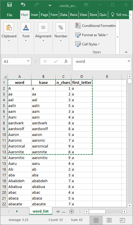
The code below shows how the data can be copied. The Windows clipboard can be used as a “file” in the read.table() tab-delimited function.
xlsclip <- read.table(file = "clipboard", sep = "\t", header = TRUE)
xlsclip %>%
kable() %>%
kable_styling(
full_width = FALSE,
position = "left"
)| word | lcase | n_chars | first_letter |
|---|---|---|---|
| A | a | 1 | a |
| aa | aa | 2 | a |
| aal | aal | 3 | a |
| aalii | aalii | 5 | a |
| aam | aam | 3 | a |
| Aani | aani | 4 | a |
| aardvark | aardvark | 8 | a |
| aardwolf | aardwolf | 8 | a |
| Aaron | aaron | 5 | a |
| Aaronic | aaronic | 7 | a |
| Aaronical | aaronical | 9 | a |
| Aaronite | aaronite | 8 | a |
9.12 Running system commands
R can run arbitrary system commands that you would normally run in a terminal or command window. The system() function is used to run commands, optionally with the results returned as a character vector. Under Mac and Linux, the usage is quite straightforward, for example, to list files in a specific directory:
tempdirfiles <- system("ls $TEMP", intern = TRUE)Under Windows, it takes a bit of extra code. To do the same requires the prefix cmd /c in the system() call before the command itself. Also any backslashes in path names need to be specified as double-backslashes for R.
library(magrittr)
# R prefers and automatically generates forward slashes
tmpdir <- dirname(tempdir())
# what is the OS
os <- .Platform$OS.type
# construct a system command
# under Windows
if (os == "windows") {
# under Windows, path delimiters are backslashes so need to be rendered in R as double backslashes
tmpdir %<>% str_replace_all("/", "\\\\")
# formulate the command
cmd <- sprintf("cmd /c dir %s", tmpdir)
# run the command
tempdirfiles <- system(command = cmd, intern = TRUE)
}
# under *NIX
if (os == "unix") {
cmd <- sprintf("ls %s", tmpdir)
tempdirfiles <- system(command = cmd, intern = TRUE)
}If you are running other programs or utilities that are executed in a terminal or command window, this can be very helpful. Use intern = TRUE to return the results of the command as an object in the R environment.
9.13 Code styling
Good code should meet at least the two functional requirements of getting the job done and being able able to read. Code that gets the job done but that is not easy to read will cause problems later when you try to figure out how or why you did something.
The styler package can help clean up your code so that it conforms to a specific style such as that in the tidyverse style guide. styler can be integrated into RStudio for interactive use. It can reformat selected code, an entire file, or an entire project. An example is shown:
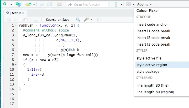
lintr is also useful for identifying potential style errors.
9.14 Session information
It may be helpful in troubleshooting or complete documentation to report the complete session information. For example, sometimes outdated versions of packages may contain errors. The session information is printed with sessionInfo().
## R version 4.1.2 (2021-11-01)
## Platform: x86_64-w64-mingw32/x64 (64-bit)
## Running under: Windows Server x64 (build 17763)
##
## Matrix products: default
##
## locale:
## [1] LC_COLLATE=English_United States.1252
## [2] LC_CTYPE=English_United States.1252
## [3] LC_MONETARY=English_United States.1252
## [4] LC_NUMERIC=C
## [5] LC_TIME=English_United States.1252
##
## attached base packages:
## [1] stats graphics grDevices utils datasets methods base
##
## other attached packages:
## [1] RVerbalExpressions_0.1.0 sf_1.0-7 htmltools_0.5.2
## [4] leaflet_2.1.0 tidycensus_1.1.2 fstcore_0.9.8
## [7] fst_0.9.8 lubridate_1.8.0 sqldf_0.4-11
## [10] RSQLite_2.2.10 gsubfn_0.7 proto_1.0.0
## [13] curl_4.3.2 haven_2.4.3 kableExtra_1.3.4.9000
## [16] knitr_1.37 magrittr_2.0.2 forcats_0.5.1
## [19] stringr_1.4.0 dplyr_1.0.8 purrr_0.3.4
## [22] readr_2.1.2 tidyr_1.2.0 tibble_3.1.6
## [25] ggplot2_3.3.5 tidyverse_1.3.1
##
## loaded via a namespace (and not attached):
## [1] fs_1.5.2 bit64_4.0.5 RColorBrewer_1.1-2 webshot_0.5.2
## [5] httr_1.4.2 tools_4.1.2 backports_1.4.1 bslib_0.3.1
## [9] rgdal_1.5-28 utf8_1.2.2 R6_2.5.1 KernSmooth_2.23-20
## [13] DBI_1.1.2 colorspace_2.0-3 sp_1.4-6 withr_2.5.0
## [17] tidyselect_1.1.2 downlit_0.4.0 bit_4.0.4 compiler_4.1.2
## [21] chron_2.3-56 cli_3.2.0 rvest_1.0.2 xml2_1.3.3
## [25] bookdown_0.24.4 sass_0.4.0 scales_1.1.1 classInt_0.4-3
## [29] proxy_0.4-26 rappdirs_0.3.3 systemfonts_1.0.4 digest_0.6.29
## [33] foreign_0.8-82 rmarkdown_2.13 svglite_2.1.0 pkgconfig_2.0.3
## [37] dbplyr_2.1.1 fastmap_1.1.0 highr_0.9 htmlwidgets_1.5.4
## [41] rlang_1.0.2 readxl_1.3.1 rstudioapi_0.13 farver_2.1.0
## [45] jquerylib_0.1.4 generics_0.1.2 jsonlite_1.8.0 crosstalk_1.2.0
## [49] Rcpp_1.0.8 munsell_0.5.0 fansi_1.0.2 lifecycle_1.0.1
## [53] stringi_1.7.6 yaml_2.3.5 maptools_1.1-3 grid_4.1.2
## [57] blob_1.2.2 parallel_4.1.2 crayon_1.5.0 lattice_0.20-45
## [61] hms_1.1.1 pillar_1.7.0 uuid_1.0-3 tcltk_4.1.2
## [65] reprex_2.0.1 glue_1.6.2 evaluate_0.15 data.table_1.14.2
## [69] modelr_0.1.8 vctrs_0.3.8 tzdb_0.2.0 cellranger_1.1.0
## [73] gtable_0.3.0 assertthat_0.2.1 cachem_1.0.6 xfun_0.30
## [77] broom_0.7.12 e1071_1.7-9 class_7.3-20 viridisLite_0.4.0
## [81] tigris_1.6 memoise_2.0.1 units_0.8-0 ellipsis_0.3.29.15 Commenting out Rmd/HTML code
To comment out entire parts of your Rmd so they do not appear in your rendered HTML, use HTML comments, which are specified with the delimiters <!-- and -->. For example, you will not see anything between these two blocks of angle brackets in the HTML output, but if you look at the complete code for the Rmd file that generated this document (below), you will get a treat.
Rendered at 2022-03-12 10:49:09.711
9.16 Source code
File is at CSDE-TS1: R:/Project/CSDE502/2022/csde502-winter-2022-main/09-week09.Rmd.
9.16.1 R code used in this document
library(tidyverse)
library(magrittr)
library(knitr)
library(kableExtra)
library(haven)
library(curl)
library(ggplot2)
# URL home
urlhome <- ""
# path to this file name
if (!interactive()) {
fnamepath <- current_input(dir = TRUE)
fnamestr <- paste0(Sys.getenv("COMPUTERNAME"), ": ", fnamepath)
} else {
fnamepath <- ""
}
paste(LETTERS[1], letters[1])
paste0(LETTERS[1], letters[1])
library(curl)
# zip file
zipfile <- file.path(tempdir(), "quickfox.zip")
# download
curl_download(url = "http://staff.washington.edu/phurvitz/csde502_winter_2021/files/quickfox.zip", destfile = zipfile)
# unzip
unzip(zipfile = zipfile, overwrite = TRUE, exdir = tempdir())
# files in the zip file
fnames <- unzip(zipfile = file.path(tempdir(), "quickfox.zip"), list = TRUE) %>%
pull(Name) %>%
file.path(tempdir(), .)
# read each file
for (i in seq_len(length(fnames))) {
# the file name with a forward slash
fname <- fnames[i] %>% normalizePath(winslash = "/")
# read the file
mytext <- scan(file = fname, what = "character", quiet = TRUE)
# vvvvvvvvvvvvvvvvvvvvvvvvvvvvvv
# make a string using `paste()` and a tab
mystr <- paste0(mytext, "\t", i, " of ", length(fnames), "; file = ", fname)
# ^^^^^^^^^^^^^^^^^^^^^^^^^^^^^^
# print the message
message(mystr)
}
# some numerical ZIP codes
(zip_bad <- data.frame(id = 1:3, zipcode = c(90201, 02134, 00501)))
# fix them up
(zip_good <- zip_bad %>%
    mutate(
        zipcode = sprintf("%05d", zipcode)
    ))
# numbers with a variety of decimal places
v <- c(1.2, 2.345, 1e+5 + 00005)

# four fixed decimal places
v %>% sprintf("%0.4f", .)
# round to 4 places
v %>% round(., 4)
# a big number
bignum <- pi * 1e+08

# commas
(us_format <- bignum %>%
        prettyNum(big.mark = ",", digits = 15)) %>%
    paste("US:", .)
# spaces, common Euro format
(euro_format1 <- bignum %>%
        prettyNum(big.mark = " ", digits = 15, decimal.mark = ",")) %>%
    paste("some Europe:", .)
# other Euro format
(euro_format2 <- bignum %>% prettyNum(big.mark = "'", digits = 15, decimal.mark = ",")) %>%
    paste("other Europe:", .)
# read each file
for (i in seq_len(length(fnames))) {
    # the file name
    fname <- fnames[i]
    # read the file
    mytext <- scan(file = fname, what = "character", quiet = TRUE)

    # vvvvvvvvvvvvvvvvvvvvvvvvvvvvvv
    # make a string using `paste()`
    mystr <- sprintf("%s\t%s of %s:\t%s\n", mytext, i, length(fnames), fname)
    # ^^^^^^^^^^^^^^^^^^^^^^^^^^^^^^

    # print the message
    cat(mystr)
}
subjects <- c("a1", "b2", "c3")

f <- function(id) {
    # create an output file name by substituting in the subject ID
    outfname <- file.path(tempdir(), "xIDx.csv") %>%
        str_replace(pattern = "xIDx", id)
    # ... do a bunch of stuff, for example
    val <- rnorm(1)
    # write the file
    message(paste0("writing subject ", id, "'s data to ", outfname))
    write.csv(x = val, file = outfname)
}

for (i in subjects) {
    f(i)
}
n_fnames <- length(fnames)
# create progress bar
pb <- txtProgressBar(min = 0, max = n_fnames, style = 3)
for (i in 1:n_fnames) {
    # delay a bit
    Sys.sleep(0.1)
    # update progress bar
    setTxtProgressBar(pb, i)
    # read and print from the file
    txt <- scan(fnames[i], what = "character", quiet = TRUE)
    cat("\n", txt, "\n")
}
close(pb)
verbose = TRUE
for (i in zip_good %>% pull(zipcode)) {
    # do some stuff
    vals <- rnorm(n = 3)
    y <- bind_cols(zipcode = i, v = vals)
    # a writing command using sprintf() to substitute %s = ZIP code
    cmd <- sprintf("write.csv(x = y, file = file.path(tempdir(), '%s.csv'), row.names = FALSE)", i)

    # show what the command is
    if(verbose){
        cat(cmd, "\n")
    }

    # this runs the command
    eval(parse(text = cmd))
}
library(sqldf)
library(kableExtra)

sqlc <- '
select
    "Species" as species
    , avg("Sepal.Length") as mean_sepal_length
    , avg("Sepal.Width") as mean_sepal_width
from iris
group by "Species";'

iris_summary <- sqldf(x = sqlc)

iris_summary %>%
    kable(caption = "Mean sepal length from the iris data set") %>%
    kable_styling(full_width = FALSE, position = "left")
iris_summary2 <- iris %>%
    group_by(Species) %>%
    summarise(
        mean_sepal_length = mean(Sepal.Length),
        mean_sepal_width = mean(Sepal.Width)) %>%
    select(species = Species, everything())

iris_summary2 %>%
    kable(caption = "Mean sepal length from the iris data set (tidyverse approach)") %>%
    kable_styling(full_width = FALSE, position = "left")
try(
    read.csv("http://staff.washington.edu/phurvitz/csde502_winter_2021/password_protected/foo.csv")
)
try(
    read.csv("http://csde:502@staff.washington.edu/phurvitz/csde502_winter_2021/password_protected/foo.csv")
)
options(digits = 22)
Sys.time() %>% as.numeric()
(eagle <- as.POSIXct(x = "7/20/69 10:56 PM", tz = "CST6CDT", format = "%m/%d/%y %H:%M"))
library(lubridate)
# set the option for fractional seconds
options(digits.secs = 3)
(now <- Sys.time() %>%
        strptime("%Y-%m-%d %H:%M:%OS"))
# show this at time zone UTC
(with_tz(time = now, tzone = "UTC"))
# in different format
now %>%
    format("%A, %B %d, %Y %l:%m %p %Z")
# reset the digits
options(digits = 7)
# mark time and run a process
t0 <- Sys.time()
# delay 5 seconds
Sys.sleep(5)
# mark the time now that the 5 second delay has run
t1 <- Sys.time()

# difftime() unqualified will make its best decision about what to print
(difftime(time1 = t1, time2 = t0))
# time between moon step and now-ish
(difftime(time1 = t0, time2 = eagle))
(difftime(time1 = t1, time2 = t0, units = "secs") %>%
     as.numeric()) %>% round(0)
(difftime(time1 = t1, time2 = t0, units = "mins") %>%
        as.numeric()) %>% round(2)
(difftime(time1 = t1, time2 = t0, units = "hours") %>%
        as.numeric()) %>% round(4)
(difftime(time1 = t1, time2 = t0, units = "days") %>%
        as.numeric()) %>% round(6)
(difftime(time1 = t1, time2 = eagle, units = "secs") %>%
     as.numeric())
(difftime(time1 = t1, time2 = eagle, units = "mins") %>%
        as.numeric())
(difftime(time1 = t1, time2 = eagle, units = "hours") %>%
        as.numeric())
(difftime(time1 = t1, time2 = eagle, units = "days") %>%
        as.numeric())
(time_length(x = difftime(time1 = t1, time2 = eagle), unit = "years") %>%
        as.numeric() %>% round(1))
library(fst)
library(haven)

myUrl <- "http://staff.washington.edu/phurvitz/csde502_winter_2021/data/21600-0001-Data.dta.zip"
# zip file in $temp
zipfile <- file.path(tempdir(), basename(myUrl))
# download
curl_download(url = myUrl, destfile = zipfile)
# dta file in $temp
dtafname <- tools::file_path_sans_ext(zipfile)
# check if the dta file exists
if (!file.exists(dtafname)) {
    # if the dta file doesn't exist, check for the zip file
    # check if the zip file exists, download if necessary
    if (!file.exists(zipfile)) {
        curl::curl_download(url = myUrl, destfile = zipfile)
    }
    # unzip the downloaded zip file
    unzip(zipfile = zipfile, exdir = tempdir())
}

# read the file
dat <- read_dta(dtafname)

# save as a CSV, along with timing
t0 <- Sys.time()
csvfname <- dtafname %>% str_replace(pattern = "dta", replacement = "csv")
write.csv(x = dat, file = csvfname, row.names = FALSE)
t1 <- Sys.time()
csvwrite_time <- difftime(time1 = t1, time2 = t0, units = "secs") %>%
    as.numeric() %>%
    round(1)

# file size
csvsize <- file.info(csvfname) %>%
    pull(size) %>%
    sprintf("%0.f", .)

# save as FST, along with timing
t0 <- Sys.time()
fstfname <- dtafname %>% str_replace(pattern = "dta", replacement = "fst")
write.fst(x = dat, path = fstfname)
t1 <- Sys.time()

# file size
fstsize <- file.info(fstfname) %>%
    pull(size) %>%
    sprintf("%0.f", .)
fstwrite_time <- difftime(time1 = t1, time2 = t0, units = "secs") %>%
    as.numeric() %>%
    round(1)
library(tidycensus)
# the census variables
census_vars <- c(
p_denom_race = "B02001_001",
p_n_white = "B02001_002",
p_n_afram = "B02001_003",
p_n_aian = "B02001_004",
p_n_asian = "B02001_005"
)
# get the data
ctdat <- get_acs(
geography = "tract",
variables = census_vars,
cache_table = TRUE,
year = 2019,
output = "wide",
state = "WA",
county = "King",
geometry = TRUE,
survey = "acs5",
progress_bar = FALSE
)
# print a few records
ctdat %>%
head() %>%
kable(caption = "Selected census tract variables from the 5-year ACS from 2019 for King County, WA") %>%
kable_styling(full_width = FALSE, position = "left")
library(leaflet)
library(htmltools)
library(sf)
# define the CRS
st_crs(ctdat) <- 4326
# proportion Black
ctdat %<>%
mutate(pct_black = (p_n_aframE / p_denom_raceE * 100) %>% round(1))
# a label
labels <- sprintf("%s<br/>%s%s", ctdat$GEOID, ctdat$pct_black, "%") %>% lapply(htmltools::HTML)
bins <- 0:50
pal <- colorBin(
palette = "Reds",
domain = ctdat$pct_black,
bins = bins
)
bins2 <- seq(0, 50, by = 10)
pal2 <- colorBin(
palette = "Reds",
domain = ctdat$pct_black,
bins = bins2
)
# the leaflet map
m <- leaflet(height = "500px") %>%
# add polygons from tracts
addPolygons(
data = ctdat,
weight = 1,
fillOpacity = 0.8,
# fill using the palette
fillColor = ~ pal(pct_black),
# highlighting
highlight = highlightOptions(
weight = 5,
color = "#666",
fillOpacity = 0.7,
bringToFront = TRUE
),
# popup labels
label = labels,
labelOptions = labelOptions(
style = list("font-weight" = "normal", padding = "3px 8px"),
textsize = "15px",
direction = "auto"
)
) %>%
# legend
addLegend(
position = "bottomright", pal = pal2, values = ctdat$pct_black,
title = "% African American",
opacity = 1
)
m %>% addTiles()
library(RVerbalExpressions)
# a pattern
x <- rx_start_of_line() %>%
rx_find("http") %>%
rx_maybe("s") %>%
rx_find("://") %>%
rx_maybe("www.") %>%
rx_anything_but(" ") %>%
rx_end_of_line()
# print the expression
(x)
# search for a pattern in some URLs
urls <- c(
"http://www.google.com",
"http://staff.washington.edu/phurvitz/csde502_winter_2021/"
)
grepl(pattern = x, x = urls)
# a different pattern
y <- rx_start_of_line() %>%
rx_find("http") %>%
rx_maybe("s") %>%
rx_find("://") %>%
rx_find("www.") %>%
rx_anything_but(" ") %>%
rx_end_of_line()
# print the expression
(y)
# search for a pattern in the two URLs, matches one, does not match the other
grepl(pattern = y, x = urls)
xlsclip <- fst::read.fst("files/xlsclip.fst")
xlsclip <- read.table(file = "clipboard", sep = "\t", header = TRUE)
xlsclip %>%
kable() %>%
kable_styling(
full_width = FALSE,
position = "left"
)
xlsclip %>%
kable() %>%
kable_styling(
full_width = FALSE,
position = "left"
)
library(magrittr)
# R prefers and automatically generates forward slashes
tmpdir <- dirname(tempdir())
# what is the OS
os <- .Platform$OS.type
# construct a system command
# under Windows
if (os == "windows") {
# under Windows, path delimiters are backslashes so need to be rendered in R as double backslashes
tmpdir %<>% str_replace_all("/", "\\\\")
# formulate the command
cmd <- sprintf("cmd /c dir %s", tmpdir)
# run the command
tempdirfiles <- system(command = cmd, intern = TRUE)
}
# under *NIX
if (os == "unix") {
cmd <- sprintf("ls %s", tmpdir)
tempdirfiles <- system(command = cmd, intern = TRUE)
}
sessionInfo()
cat(readLines(fnamepath), sep = '\n')9.16.2 Complete Rmd code
# Week 9 {#week9}
```{r, echo=FALSE, warning=FALSE, message=FALSE}
library(tidyverse)
library(magrittr)
library(knitr)
library(kableExtra)
library(haven)
library(curl)
library(ggplot2)
# URL home
urlhome <- ""
# path to this file name
if (!interactive()) {
fnamepath <- current_input(dir = TRUE)
fnamestr <- paste0(Sys.getenv("COMPUTERNAME"), ": ", fnamepath)
} else {
fnamepath <- ""
}
```
<h2>Topic: Miscellaneous data processing </h2>
This week's lesson will cover a set of miscellaneous data processing topics that can be useful in different situations.
Mostly this is a set of coded examples with explanations.
Download [template.Rmd.txt](files/template.Rmd.txt) as a template for this lesson. Save in in your working folder for the course, renamed to `week_09.Rmd` (with no `.txt` extension). Make any necessary changes to the YAML header.
## Substituting text
### `paste()`, `paste0()`
Pasting text allows you to substitute variables within a text string. For example, if you are running a long loop over a series of files and you want to know which file name and loop iteration you are on.
The function `paste()` combines a set of strings and adds a space between the strings, e.g., combining the first values from the `LETTERS` and the `letters` built-in vectors:
```{r}
paste(LETTERS[1], letters[1])
```
whereas `paste0` does not add spaces:
```{r}
paste0(LETTERS[1], letters[1])
```
The code below uses the function `tempdir()` to specify a folder that is automatically generated per R session; for this rendering of the book, the location was ``r tempdir()`` but will almost certainly be different for your session. The code downloads and unzips the file [quickfox](files/quickfox.zip) to the `tempdir()` location. The zip file contains a separate file for each word in the phrase "the quick brown fox jumps over the lazy dog". The code then uses a loop and `paste0()` to show the contents of each separate file along with its file name.
```{r}
library(curl)
# zip file
zipfile <- file.path(tempdir(), "quickfox.zip")
# download
curl_download(url = "http://staff.washington.edu/phurvitz/csde502_winter_2021/files/quickfox.zip", destfile = zipfile)
# unzip
unzip(zipfile = zipfile, overwrite = TRUE, exdir = tempdir())
# files in the zip file
fnames <- unzip(zipfile = file.path(tempdir(), "quickfox.zip"), list = TRUE) %>%
pull(Name) %>%
file.path(tempdir(), .)
# read each file
for (i in seq_len(length(fnames))) {
# the file name with a forward slash
fname <- fnames[i] %>% normalizePath(winslash = "/")
# read the file
mytext <- scan(file = fname, what = "character", quiet = TRUE)
# vvvvvvvvvvvvvvvvvvvvvvvvvvvvvv
# make a string using `paste()` and a tab
mystr <- paste0(mytext, "\t", i, " of ", length(fnames), "; file = ", fname)
# ^^^^^^^^^^^^^^^^^^^^^^^^^^^^^^
# print the message
message(mystr)
}
```
### `sprintf()`
`sprintf()` can be used to format text. Here are just a few examples. The result is a formatted text string.
#### Formatting numerical values
<u>Leading zeros</u>
Numeric values can be formatted as character strings with a specific number of decimal places or leading zeros. For example, ZIP codes imported from CSV files often are converted to integers. The following code chunk converts some numerical ZIP code-like values to text values with the correct format.
Bad ZIP codes; the 5-digit numerical values are read in as double-precision numbers, so the leading zeros are dropped:
```{r}
# some numerical ZIP codes
(zip_bad <- data.frame(id = 1:3, zipcode = c(90201, 02134, 00501)))
```
Good ZIP codes:
```{r}
# fix them up
(zip_good <- zip_bad %>%
mutate(
zipcode = sprintf("%05d", zipcode)
))
```
The `sprintf()` format `%05d` indicates that if the input string is less than 5 characters in length, then make the output string 5 characters and pad on the left with zeros.
<u>Decimal places</u>
Numerical values with different numbers of decimal places can be rendered with a specific number of decimal places.
```{r}
# numbers with a variety of decimal places
v <- c(1.2, 2.345, 1e+5 + 00005)
# four fixed decimal places
v %>% sprintf("%0.4f", .)
```
Note that this is distinct from `round()`, which results in a numeric vector:
```{r}
# round to 4 places
v %>% round(., 4)
```
<u>Commas or spaces for large numbers</u>
Particularly in the narrative, including formatted numbers is important for readability based on the audience. For this, `prettyNum()` can be used. Here are a few examples:
```{r}
# a big number
bignum <- pi * 1e+08
# commas
(us_format <- bignum %>%
prettyNum(big.mark = ",", digits = 15)) %>%
paste("US:", .)
# spaces, common Euro format
(euro_format1 <- bignum %>%
prettyNum(big.mark = " ", digits = 15, decimal.mark = ",")) %>%
paste("some Europe:", .)
# other Euro format
(euro_format2 <- bignum %>% prettyNum(big.mark = "'", digits = 15, decimal.mark = ",")) %>%
paste("other Europe:", .)
```
This literal text:
```
For example, used in inline code:
"$\pi$ multiplied by `r format(1e+8, scientific = FALSE)`
equals approximately `r us_format`."
```
appears as:
For example, used in inline code: "$\pi$ multiplied by `r `format(1e+8, scientific = FALSE)` equals approximately `r us_format`."
#### String substitutions
`sprintf()` can also be used to achieve the same substitution in the file reading loop above. Each `%s` is substituted in order of the position of the arguments following the string. Also note that `\t` inserts a `TAB` character.
```{r}
# read each file
for (i in seq_len(length(fnames))) {
# the file name
fname <- fnames[i]
# read the file
mytext <- scan(file = fname, what = "character", quiet = TRUE)
# vvvvvvvvvvvvvvvvvvvvvvvvvvvvvv
# make a string using `paste()`
mystr <- sprintf("%s\t%s of %s:\t%s\n", mytext, i, length(fnames), fname)
# ^^^^^^^^^^^^^^^^^^^^^^^^^^^^^^
# print the message
cat(mystr)
}
```
### `str_replace()`, `str_replace_all()`
The `stringr` functions `str_replace()` and `str_replace_all()` can be used to substitute specific strings in other strings. For example, we might create a generic function to run over a set of subject IDs that generates a file for each subject.
```{r}
subjects <- c("a1", "b2", "c3")
f <- function(id) {
# create an output file name by substituting in the subject ID
outfname <- file.path(tempdir(), "xIDx.csv") %>%
str_replace(pattern = "xIDx", id)
# ... do a bunch of stuff, for example
val <- rnorm(1)
# write the file
message(paste0("writing subject ", id, "'s data to ", outfname))
write.csv(x = val, file = outfname)
}
for (i in subjects) {
f(i)
}
```
## Showing progress
A text-based progress bar can be shown using the `txtProgressBar()`. Here we run the same loop for reading the text files, but rather than printing the loop iteration and file names, we show the progress bar and the file contents. If no text is printed to the console (unlike what is demonstrated below with `cat()`), the progress bar will not print on several lines.
It is generally not recommended to put a progress bar in an R Markdown document since the output is usually read as a static file. However, progress bars may be helpful in `shiny` R Markdown documents if a process will take longer than a few seconds.
```{r}
n_fnames <- length(fnames)
# create progress bar
pb <- txtProgressBar(min = 0, max = n_fnames, style = 3)
for (i in 1:n_fnames) {
# delay a bit
Sys.sleep(0.1)
# update progress bar
setTxtProgressBar(pb, i)
# read and print from the file
txt <- scan(fnames[i], what = "character", quiet = TRUE)
cat("\n", txt, "\n")
}
close(pb)
```
For other implementations of progress bars, see [progress: Terminal Progress Bars
](https://cran.r-project.org/web/packages/progress).
## Turning text into code: `eval(parse(text = "some string"))`
Sometimes you may have variables whose values that you want to use in a command or function. For example, suppose you wanted to write a set of files, one for each ZIP code in a data frame, with a file name including the ZIP code. We would not want to use the column name `zipcode`, but we want the actual values in the column.
We can generate a string that represents a command using the same kind of text substitution as above with `sprintf()`. The loop processes each ZIP code record, `pull()`ing the ZIP code value at each iteration. A `write.csv()` command is generated for each iteration, setting the output file name to include the current iteration's ZIP code.
Finally, the last step in each iteration is `eval(parse(text = cmd))` which executes the `cmd` string as a command.
```{r}
verbose = TRUE
for (i in zip_good %>% pull(zipcode)) {
# do some stuff
vals <- rnorm(n = 3)
y <- bind_cols(zipcode = i, v = vals)
# a writing command using sprintf() to substitute %s = ZIP code
cmd <- sprintf("write.csv(x = y, file = file.path(tempdir(), '%s.csv'), row.names = FALSE)", i)
# show what the command is
if(verbose){
cat(cmd, "\n")
}
# this runs the command
eval(parse(text = cmd))
}
```
## SQL in R with `RSQLite` and `sqldf`
Sometimes R's syntax for processing data can be difficult and confusing. For programmers who are familiar with structured query language (SQL), it is possible to run SQL statements within R using a supported database back end (by default SQLite) and the `sqldf()` function.
For example, the mean sepal length by species from the built-in `iris` data set can be obtained, presented in Tables \@ref(tab:iris) and \@ref(tab:iris2).
```{r iris, message=FALSE}
library(sqldf)
library(kableExtra)
sqlc <- '
select
"Species" as species
, avg("Sepal.Length") as mean_sepal_length
, avg("Sepal.Width") as mean_sepal_width
from iris
group by "Species";'
iris_summary <- sqldf(x = sqlc)
iris_summary %>%
kable(caption = "Mean sepal length from the iris data set") %>%
kable_styling(full_width = FALSE, position = "left")
```
This would be equivalent in `tidyverse` as
```{r iris2, message=FALSE}
iris_summary2 <- iris %>%
group_by(Species) %>%
summarise(
mean_sepal_length = mean(Sepal.Length),
mean_sepal_width = mean(Sepal.Width)) %>%
select(species = Species, everything())
iris_summary2 %>%
kable(caption = "Mean sepal length from the iris data set (tidyverse approach)") %>%
kable_styling(full_width = FALSE, position = "left")
```
## Downloading files from password-protected web sites
Some web sites are protected by simple username/password protection. For example, try opening http://staff.washington.edu/phurvitz/csde502_winter_2021/password_protected/foo.csv. The username/password pair is csde/502, which will allow you to see the contents of the web folder.
If you try downloading the file through R, you will get an error because no password is supplied.
```{r}
try(
read.csv("http://staff.washington.edu/phurvitz/csde502_winter_2021/password_protected/foo.csv")
)
```
However, the username and password can be supplied as part of the URL, as below. When the username and password are supplied, they will be cached for that site for the duration of the R session (so if you try running this again, you will succeed without a password).
```{r}
try(
read.csv("http://csde:502@staff.washington.edu/phurvitz/csde502_winter_2021/password_protected/foo.csv")
)
```
## Dates and time stamps: `POSIXct` and `lubridate`
R uses POSIX-style time stamps, which are stored internally as the number of fractional seconds from January 1, 1970. It is imperative that the control over time stamps is commensurate with the temporal accuracy and precision your data. For example, in the measurement of years of residence, precision is not substantially important. For measurement of chemical reactions, fractional seconds may be very important. For applications such as merging body-worn sensor data from GPS units and accelerometers for estimating where and when physical activity occurs, minutes of error can result in statistically significant mis-estimations.
For example, you can see the numeric value of these seconds as `options(digits = 22); Sys.time() %>% as.numeric()`.
```{r}
options(digits = 22)
Sys.time() %>% as.numeric()
```
If you have time stamps in text format, they can be converted to POSIX time stamps, e.g., the supposed time Neil Armstrong stepped on the moon:
```{r}
(eagle <- as.POSIXct(x = "7/20/69 10:56 PM", tz = "CST6CDT", format = "%m/%d/%y %H:%M"))
```
Formats can be specified using specific codes, see `strptime()`.
The `lubridate` package has a large number of functions for handling date and time stamps. For example, if you want to convert a time stamp in the current time zone to a different time zone, first we get the current time
```{r, message=FALSE}
library(lubridate)
# set the option for fractional seconds
options(digits.secs = 3)
(now <- Sys.time() %>%
strptime("%Y-%m-%d %H:%M:%OS"))
```
And convert to UTC:
```{r}
# show this at time zone UTC
(with_tz(time = now, tzone = "UTC"))
```
or show in a different format:
```{r}
# in different format
now %>%
format("%A, %B %d, %Y %l:%m %p %Z")
```
```{r, echo=FALSE}
# reset the digits
options(digits = 7)
```
## Timing with `Sys.time()` and `difftime()`
It is easy to determine how long a process takes by using sequential `Sys.time()` calls, one before and one after the process, and getting the difference with `difftime()`. For example,
```{r}
# mark time and run a process
t0 <- Sys.time()
# delay 5 seconds
Sys.sleep(5)
# mark the time now that the 5 second delay has run
t1 <- Sys.time()
# difftime() unqualified will make its best decision about what to print
(difftime(time1 = t1, time2 = t0))
# time between moon step and now-ish
(difftime(time1 = t0, time2 = eagle))
```
`difftime()` can also be forced to report the time difference in the units of choice. Here is the `difftime()` from the 5-second delay we created above:
```{r}
(difftime(time1 = t1, time2 = t0, units = "secs") %>%
as.numeric()) %>% round(0)
(difftime(time1 = t1, time2 = t0, units = "mins") %>%
as.numeric()) %>% round(2)
(difftime(time1 = t1, time2 = t0, units = "hours") %>%
as.numeric()) %>% round(4)
(difftime(time1 = t1, time2 = t0, units = "days") %>%
as.numeric()) %>% round(6)
```
... and the time since the Eagle had landed to now:
```{r}
(difftime(time1 = t1, time2 = eagle, units = "secs") %>%
as.numeric())
(difftime(time1 = t1, time2 = eagle, units = "mins") %>%
as.numeric())
(difftime(time1 = t1, time2 = eagle, units = "hours") %>%
as.numeric())
(difftime(time1 = t1, time2 = eagle, units = "days") %>%
as.numeric())
```
In order to report intervals as years, use `lubridate::time_length()`:
```{r}
(time_length(x = difftime(time1 = t1, time2 = eagle), unit = "years") %>%
as.numeric() %>% round(1))
```
## Faster files with `fst()`
The `fst` package is great for rapid reading and writing of data frames. The format can also result in much smaller file sizes using compression. Here we will examine the large Add Health file. First, a download, unzip, and read as necessary:
```{r}
library(fst)
library(haven)
myUrl <- "http://staff.washington.edu/phurvitz/csde502_winter_2021/data/21600-0001-Data.dta.zip"
# zip file in $temp
zipfile <- file.path(tempdir(), basename(myUrl))
# download
curl_download(url = myUrl, destfile = zipfile)
# dta file in $temp
dtafname <- tools::file_path_sans_ext(zipfile)
# check if the dta file exists
if (!file.exists(dtafname)) {
# if the dta file doesn't exist, check for the zip file
# check if the zip file exists, download if necessary
if (!file.exists(zipfile)) {
curl::curl_download(url = myUrl, destfile = zipfile)
}
# unzip the downloaded zip file
unzip(zipfile = zipfile, exdir = tempdir())
}
# read the file
dat <- read_dta(dtafname)
# save as a CSV, along with timing
t0 <- Sys.time()
csvfname <- dtafname %>% str_replace(pattern = "dta", replacement = "csv")
write.csv(x = dat, file = csvfname, row.names = FALSE)
t1 <- Sys.time()
csvwrite_time <- difftime(time1 = t1, time2 = t0, units = "secs") %>%
as.numeric() %>%
round(1)
# file size
csvsize <- file.info(csvfname) %>%
pull(size) %>%
sprintf("%0.f", .)
# save as FST, along with timing
t0 <- Sys.time()
fstfname <- dtafname %>% str_replace(pattern = "dta", replacement = "fst")
write.fst(x = dat, path = fstfname)
t1 <- Sys.time()
# file size
fstsize <- file.info(fstfname) %>%
pull(size) %>%
sprintf("%0.f", .)
fstwrite_time <- difftime(time1 = t1, time2 = t0, units = "secs") %>%
as.numeric() %>%
round(1)
```
It took `r csvwrite_time` s to write `r csvsize` bytes as CSV, and `r fstwrite_time` s to write `r fstsize` bytes as a FST file (with the default compression amount of 50). Reading speeds are comparable.
___It should be noted___ that some file attributes will not be saved in FST format and therefore it should be used with caution if you have a highly attributed data set (e.g., a Stata DTA file with extensive labeling, or a data frame with a lot of customized attribute labels). You will lose those attributes! But for data sets with a simple structure, including factors, the FST format is a good option. With a little work, the attributes of a data frame could be saved as a list (e.g., as an `.RData` file along with the `.fst` file) and then applied after the `.fst` file is loaded.
## Load US Census Boundary and Attribute Data as 'tidyverse' and 'sf'-Ready Data Frames: `tigris`, `tidycensus`
*[This has been covered previously, but is included here as a quick recap; skip to [RVerbalExpressions](#rverbalexpressions).]*
Dealing with US Census data can be overwhelming, particularly if using the raw text-based data. The Census Bureau has an API that allows more streamlined downloads of variables (as data frames) and geographies (as simple format shapes). It is necessary to get an API key, available for free. See [tidycensus](https://walker-data.com/tidycensus/) and [tidycensus basic usage](https://walker-data.com/tidycensus/articles/basic-usage.html).
`tidycensus` uses [`tigris`](https://www.rdocumentation.org/packages/tigris/versions/1.0), which downloads the geographic data portion of the census files.
### Download data
A simple example will download the variables representing the count of White, Black/African American, American Indian/Native American, and Asian persons from the American Community Survey (ACS) data for King County in 2019. For this example to run, you need to have your US Census API key installed, e.g.,
<tt>
tidycensus::census_api_key("*****************", install = TRUE)<br>
<font color="red">
Your API key has been stored in your .Renviron and can be accessed by Sys.getenv("CENSUS_API_KEY").<br>
To use now, restart R or run `readRenviron("~/.Renviron")`
</font>
</tt>
The labels from the census API are:
```
"Estimate!!Total"
"Estimate!!Total!!White alone"
"Estimate!!Total!!Black or African American alone"
"Estimate!!Total!!American Indian and Alaska Native alone"
"Estimate!!Total!!Asian alone"
```
```{r, warning=FALSE, message=FALSE}
library(tidycensus)
# the census variables
census_vars <- c(
    p_denom_race = "B02001_001",
    p_n_white = "B02001_002",
    p_n_afram = "B02001_003",
    p_n_aian = "B02001_004",
    p_n_asian = "B02001_005"
)

# get the data
ctdat <- get_acs(
    geography = "tract",
    variables = census_vars,
    cache_table = TRUE,
    year = 2019,
    output = "wide",
    state = "WA",
    county = "King",
    geometry = TRUE,
    survey = "acs5",
    progress_bar = FALSE
)
```
A few values are shown in Table \@ref(tab:census)
```{r census}
# print a few records
ctdat %>%
    head() %>%
    kable(caption = "Selected census tract variables from the 5-year ACS from 2019 for King County, WA") %>%
    kable_styling(full_width = FALSE, position = "left")
```
### Mapping census data
A `leaflet` simple map is shown in \@ref(fig:ct), with percent African American residents and tract identifier.
```{r ct, fig.cap="Percent African American in census tracts in King County, 2019 ACS 5-year estimate", warning=FALSE, message=FALSE}
library(leaflet)
library(htmltools)
library(sf)

# define the CRS
st_crs(ctdat) <- 4326

# proportion Black
ctdat %<>%
    mutate(pct_black = (p_n_aframE / p_denom_raceE * 100) %>% round(1))

# a label
labels <- sprintf("%s<br/>%s%s", ctdat$GEOID, ctdat$pct_black, "%") %>% lapply(htmltools::HTML)

bins <- 0:50
pal <- colorBin(
    palette = "Reds",
    domain = ctdat$pct_black,
    bins = bins
)

bins2 <- seq(0, 50, by = 10)
pal2 <- colorBin(
    palette = "Reds",
    domain = ctdat$pct_black,
    bins = bins2
)

# the leaflet map
m <- leaflet(height = "500px") %>%
    # add polygons from tracts
    addPolygons(
        data = ctdat,
        weight = 1,
        fillOpacity = 0.8,
        # fill using the palette
        fillColor = ~ pal(pct_black),
        # highlighting
        highlight = highlightOptions(
            weight = 5,
            color = "#666",
            fillOpacity = 0.7,
            bringToFront = TRUE
        ),
        # popup labels
        label = labels,
        labelOptions = labelOptions(
            style = list("font-weight" = "normal", padding = "3px 8px"),
            textsize = "15px",
            direction = "auto"
        )
    ) %>%
    # legend
    addLegend(
        position = "bottomright", pal = pal2, values = ctdat$pct_black,
        title = "% African American",
        opacity = 1
    )
m %>% addTiles()
```
### Creating population pyramids from census data
See [Estimates of population characteristics](https://walker-data.com/tidycensus/articles/other-datasets.html#estimates-of-population-characteristics-1).
Refer also back to CSDE 533 Week 2 age structure; Week 7 interpreting age structure.
## Easier regular expressions with `RVerbalExpressions` {#rverbalexpressions}
Regular expressions are powerful but take some time and trial-and-error to master. The `RVerbalExpresions` package can be used to more easily generate regular expressions. See the help for `rx()` and associated functions.
These examples show two constructions of regular expressions for matching two similar but different URLs. First we build a regex using easy-to-understand controls:
```{r}
library(RVerbalExpressions)
# a pattern
x <- rx_start_of_line() %>%
    rx_find("http") %>%
    rx_maybe("s") %>%
    rx_find("://") %>%
    rx_maybe("www.") %>%
    rx_anything_but(" ") %>%
    rx_end_of_line()

# print the expression
(x)
```
That regex is then used to try matching against two URLs:
```{r}
# search for a pattern in some URLs
urls <- c(
    "http://www.google.com",
    "http://staff.washington.edu/phurvitz/csde502_winter_2021/"
)
grepl(pattern = x, x = urls)
```
We can try a slightly different regex pattern. The former pattern used the less strict `rx_maybe("www.")`, whereas the following pattern uses the more strict `rx_find("www.")`.
```{r}
# a different pattern
y <- rx_start_of_line() %>%
    rx_find("http") %>%
    rx_maybe("s") %>%
    rx_find("://") %>%
    rx_find("www.") %>%
    rx_anything_but(" ") %>%
    rx_end_of_line()

# print the expression
(y)
# search for a pattern in the two URLs, matches one, does not match the other
grepl(pattern = y, x = urls)
```
## Quick copy from Excel (Windows only)
Under Windows, it is possible to copy selected cells from an Excel worksheet directly to R. This is not an endorsement for using Excel, but there are some cases in which Excel may be able to produce some quick data that you don't want to develop in other ways.
As a demonstration, you can use [analysis.xlsx](files/words_analysis.xlsx). Download and open the file. Select and copy a block of cells. Here is shown a selection of cells that was copied for this example.

The code below shows how the data can be copied. The Windows clipboard can be used as a "file" in the `read.table()` tab-delimited function.
```{r, echo=FALSE}
xlsclip <- fst::read.fst("files/xlsclip.fst")
```
```{r, eval=FALSE}
xlsclip <- read.table(file = "clipboard", sep = "\t", header = TRUE)

xlsclip %>%
    kable() %>%
    kable_styling(
        full_width = FALSE,
        position = "left"
    )
```
```{r, echo=FALSE}
xlsclip %>%
kable() %>%
kable_styling(
full_width = FALSE,
position = "left"
)
```
## Running system commands
R can run arbitrary system commands that you would normally run in a terminal or command window. The `system()` function is used to run commands, optionally with the results returned as a character vector. Under Mac and Linux, the usage is quite straightforward, for example, to list files in a specific directory:
```
tempdirfiles <- system("ls $TEMP", intern = TRUE)
```
Under Windows, it takes a bit of extra code. To do the same requires the prefix `cmd /c` in the `system()` call before the command itself. Also any backslashes in path names need to be specified as double-backslashes for R.
```{r}
library(magrittr)
# R prefers and automatically generates forward slashes
tmpdir <- dirname(tempdir())

# what is the OS
os <- .Platform$OS.type

# construct a system command
# under Windows
if (os == "windows") {
    # under Windows, path delimiters are backslashes so need to be rendered in R as double backslashes
    tmpdir %<>% str_replace_all("/", "\\\\")
    # formulate the command
    cmd <- sprintf("cmd /c dir %s", tmpdir)
    # run the command
    tempdirfiles <- system(command = cmd, intern = TRUE)
}

# under *NIX
if (os == "unix") {
    cmd <- sprintf("ls %s", tmpdir)
    tempdirfiles <- system(command = cmd, intern = TRUE)
}
```
If you are running other programs or utilities that are executed in a terminal or command window, this can be very helpful. Use `intern = TRUE` to return the results of the command as an object in the R environment.
## Code styling
Good code should meet at least the two functional requirements of getting the job done and being able able to read. Code that gets the job done but that is not easy to read will cause problems later when you try to figure out how or why you did something.
The [`styler`](https://github.com/r-lib/styler) package can help clean up your code so that it conforms to a specific style such as that in the [tidyverse style guide](https://style.tidyverse.org/). `styler` can be integrated into RStudio for interactive use. It can reformat selected code, an entire file, or an entire project. An example is shown:

[`lintr`](https://github.com/jimhester/lintr) is also useful for identifying potential style errors.
## Session information
It may be helpful in troubleshooting or complete documentation to report the complete session information. For example, sometimes outdated versions of packages may contain errors. The session information is printed with `sessionInfo()`.
```{r}
sessionInfo()
```
## Commenting out Rmd/HTML code
To comment out entire parts of your Rmd so they do not appear in your rendered HTML, use HTML comments, which are specified with the delimiters `<!--` and `-->`. For example, you will not see anything between these two blocks of angle brackets in the HTML output, but if you look at the complete code for the Rmd file that generated this document (below), you will get a treat.
<!--
from https://www.gnu.org/fun/jokes/error-haiku.txt:
IMAGINE IF INSTEAD OF CRYPTIC TEXT STRINGS,
YOUR COMPUTER PRODUCED ERROR MESSAGES IN HAIKU...
A file that big?
It might be very useful.
But now it is gone.
- - - - - - - - - - - -
Yesterday it worked
Today it is not working
Windows is like that
- - - - - - - - - - - -
Stay the patient course
Of little worth is your ire
The network is down
- - - - - - - - - - - -
Three things are certain:
Death, taxes, and lost data.
Guess which has occurred.
- - - - - - - - - - - -
You step in the stream,
but the water has moved on.
This page is not here.
- - - - - - - - - - - -
Out of memory.
We wish to hold the whole sky,
But we never will.
- - - - - - - - - - - -
Having been erased,
The document you're seeking
Must now be retyped.
- - - - - - - - - - - -
Rather than a beep
Or a rude error message,
These words: "File not found."
- - - - - - - - - - - -
Serious error.
All shortcuts have disappeared.
Screen. Mind. Both are blank.
- - - - - - - - - - - -
The Web site you seek
cannot be located but
endless more exist.
- - - - - - - - - - - -
Chaos reigns within.
Reflect, repent, and reboot.
Order shall return.
- - - - - - - - - - - -
ABORTED effort:
Close all that you have.
You ask way too much.
- - - - - - - - - - - -
First snow, then silence.
This thousand dollar screen dies
so beautifully.
- - - - - - - - - - - -
With searching comes loss
and the presence of absence:
"My Novel" not found.
- - - - - - - - - - - -
The Tao that is seen
Is not the true Tao, until
You bring fresh toner.
- - - - - - - - - - - -
Windows NT crashed.
I am the Blue Screen of Death.
No one hears your screams.
- - - - - - - - - - - -
A crash reduces
your expensive computer
to a simple stone.
- - - - - - - - - - - -
Error messages
cannot completely convey.
We now know shared loss.
-- Anonymous Author
-->
<hr>
Rendered at <tt>`r Sys.time()`</tt>
## Source code
File is at `r fnamestr`.
### R code used in this document
```{r ref.label=knitr::all_labels(), echo=TRUE, eval=FALSE}
```
### Complete Rmd code
```{r comment=''}
cat(readLines(fnamepath), sep = '\n')
```